| Introduction to MATLAB |
Maple is only one of a number of computer programs that do mathematics. This course concentrates on Maple because Maple is both powerful and widely available on the Texas A&M University campus.
The best known competitor to Maple is Mathematica (at version 4.1 as of fall 2001), from Wolfram Research. Although this program is not generally available at Texas A&M University, it is available on the main Department of Mathematics server.
The program MATLAB (which stands for MATrix LABoratory) is another tool for numerical and graphical analysis. MATLAB is not a general-purpose tool, but it does a good job on what it attempts to do. It does not have built-in capabilities for symbolic calculation, but it can interface with Maple for such computations. It is a popular tool for engineering applications.
MATLAB is available on the computer systems operated by the Department of Mathematics at Texas A&M University. If you cannot find the program on a menu, you can start the program by opening a terminal window and executing the command "matlab &". When the program starts up, it will display a "Command Window" where you can type MATLAB commands.
Try a few numerical calculations. For example, try typing
2+3 and pressing Return. Notice that MATLAB (unlike Maple) requires no punctuation character to terminate
the command (indeed, MATLAB uses a semicolon as a signal to
suppress the output!) MATLAB knows all standard mathematical
functions. Try sqrt(exp(cos(log(2*pi/3)))) for example;
you should get the answer 1.4470.
There is online help available either from the "Launch Pad"
window or from the "Command Window" (type "help").
of help topics. For example, there is a topic
matlab/elfun, and typing "help matlab/elfun"
gives a list of elementary functions known to MATLAB. By
typing "help acot", you can confirm that acot is
the inverse cotangent function. There is also a command
lookfor that does a keyword search of the help files.
MATLAB deals well with arrays and matrices; indeed, MATLAB was originally written to do linear algebra. If you set
a=[1,2,3,4] and b=[5,7,11,13], then you will get
the natural componentwise results from 2*a and a+b
and sin(b). A special "dot notation" is used for
componentwise multiplication and exponentiation: try
a.*b and b.^2 and a.^b for example.
MATLAB will complain if you try to multiply a*b because
the dimensions are not right for matrix multiplication, but you
can multiply a times the transpose of b via a*b'
(try it).
Look how easy it is to implement a Caesar cipher with shift 5 in MATLAB:
     >> myword='supercalifragilisticexpialidocious'

     myword =

     supercalifragilisticexpialidocious

     >> secretword=setstr(rem(myword+5-97,26)+97)

     secretword =

     xzujwhfqnkwflnqnxynhjcunfqnithntzx

     >> undecodedword=setstr(rem(secretword-5-97+26,26)+97)

     undecodedword =

     supercalifragilisticexpialidocious
Explanation: MATLAB automatically converts the letters in a
string to their ASCII decimal equivalents if the string is
used in a numeric context. Since the letters "a" to "z" are
in ASCII positions 97 through 122, subtracting 97
translates to the range 0 to 25. Adding 5 applies
the shift, and taking the remainder upon division by 26 via
the function rem reduces modulo 26. Adding 97
translates back to the range 97 to 122, and applying
the setstr function converts back to an alphabetic
string. Reversing the operations decodes the message.
Exercise
Improve this MATLAB implementation of the Caesar cipher.Now suppose you want to make a plot. Since MATLAB is numerically oriented, you have to feed it a list of numbers (rather than the name of a function). For example, you could say x=[0, 0.2, 0.4, 0.6, 0.8, 1] and then y=cos(x) and then plot(x,y). This creates a rough plot of the cosine function on the interval from 0 to 1. The plot should pop up in a separate window.
Maybe you really wanted a plot of the cosine function on the interval from 0 to pi. Try x=x*pi and y=cos(x) and plot(x,y). Notice that MATLAB displays the new plot in the same window as before, discarding the previous plot. You can discard the plot window either by using the normal method in your operating system to kill windows or by issuing the command "close" in the "Command Window".
The preceding plots are crude because they use a small number of data points. Try x=linspace(0,pi,101); (notice the semicolon to suppress the output) to define x to be a linearly spaced partition of the interval (0,pi) into 100 subintervals, and then y=cos(x); and plot(x,y) to get a smoother plot. Try z=sin(x); and plot(x,y,x,z) to plot two functions on the same graph. What does plot(y,x) do?
You can make the graph fancy in various ways. Try some of the following.
plot(x,y,'r',x,z,'g')The predefined colors are yellow, magenta, cyan, red, green, blue, white, and black.
plot(x,y,'g:',x,z,'r-')This specifies both the colors and the characters used to mark points on the plots.
plot(x,y,'bo',x,z,'mx')
Try "help plot" to get a list of the line styles and
markers, or look in the online help available from the
"Launch Pad" window.
The command "grid" toggles grid lines on and off. The commands "axis off" and "axis on" toggle the axes. You can add labels to the plot via the commands xlabel('this labels the x axis') and ylabel('this labels the y axis') and title('this is a title'). You can also place text on the plot interactively by issuing the command gtext('some text'), moving the mouse to the appropriate spot in the plot window, and clicking the mouse.
If you set "zoom on", then you can expand or contract the plot with mouse clicks.
Here are a few examples of commands to make three-dimensional plots in MATLAB.
     x=-2:0.1:2; y=x; [X,Y]=meshgrid(x,y); % define planar grid

     Z=sin(X.*Y); % define a function

     mesh(X,Y,Z) % plot function wireframe style

     surf(X,Y,Z) % plot function patch style

     waterfall(X,Y,Z)

     colormap(gray),surfl(X,Y,Z),shading interp
For more about three-dimensional plots, try "help matlab/graph3d".
Although MATLAB lacks a fancy worksheet interface, it does
support scripts, which MATLAB calls "M-files." If you are
trying to debug a MATLAB program, you can put your MATLAB commands in a text file with extension ".m". When you
type the name of the file (without the extension) at the
command prompt in a MATLAB session, MATLAB will execute the
commands in the file as if you had typed them at the prompt.
For example, the following is a MATLAB M-file named fractal.m. If you save this file to disk and then type "fractal" in a MATLAB session, MATLAB will execute the commands to plot a fractal fern. The following commands are MATLAB equivalents of the Maple commands described in the example in the section on fractals.
%% MATLAB M-file fractal.m
iterations=25000;
Mat1=[0 0;0 0.16];
Mat2=[0.85 0.04;-0.04 0.85];
Mat3=[0.2 -0.26;0.23 0.22];
Mat4=[-0.15 0.28;0.26 0.24];
Vector1=[0;0];
Vector2=[0;1.6];
Vector3=[0;1.6];
Vector4=[0;0.44];
Prob1=0.01;
Prob2=0.85;
Prob3=0.07;
Prob4=0.07;
P=[0;0];
starttime=cputime;
for counter = 1:iterations
  prob=rand;
  if prob<Prob1
     P=Mat1*P+Vector1;
  elseif prob<Prob1+Prob2
     P=Mat2*P+Vector2;
  elseif prob<Prob1+Prob2+Prob3
     P=Mat3*P+Vector3;
  else
     P=Mat4*P+Vector4;
  end
x(counter)=P(1);
y(counter)=P(2);
end
plot(x,y,'g.')
axis equal; axis off;
title([int2str(iterations),' iterations'],'Color','red','FontSize',24);
elapsedtime=cputime-starttime;
fprintf('Execution time was %g seconds.\n', elapsedtime)
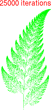 MATLAB took less than a minute
to compute the fractal fern shown in
the illustration.
Maple, on the other hand, took over a quarter of an hour to
perform the same calculation.
MATLAB took less than a minute
to compute the fractal fern shown in
the illustration.
Maple, on the other hand, took over a quarter of an hour to
perform the same calculation.
MATLAB is produced by The MathWorks, which maintains a list of books about using MATLAB and teaching mathematics with MATLAB. Also available is an archive of M-files contributed by users.
To learn more online about the capabilities of MATLAB, issue
the command "demo" in the MATLAB "Command Window" or
select "Demos" from the MATLAB "Launch Pad". To exit
MATLAB, you can type "quit" in the "Command Window".
| Introduction to MATLAB |