Determinants
Permutations
A permutation of 1, 2, ..., n is a rearrangement of these integers. For example, (3 2 4 1) is a permutation of (1 2 3 4). We will let perm(n) be the permutations of the integers 1 through n. There are n! permutations in perm(n). In the case n = 4, there are twenty-four permutations, which we list in the table below.
Permutations in perm(4)
| (1 2 3 4) | (4 1 2 3) | (3 4 1 2) |
(2 3 4 1) |
| (1 2 4 3) | (3 1 2 4) | (4 3 1 2) |
(2 4 3 1) |
| (1 3 4 2) | (2 1 3 4) | (4 2 1 3) | (3 4 2 1) |
| (1 3 2 4) | (4 1 3 2) | (2 4 1 3) |
(3 2 4 1) |
| (1 4 2 3) | (3 1 4 2) | (2 3 1 4) |
(4 2 3 1) |
| (1 4 3 2) | (2 1 4 3) | (3 2 1 4) | (4 3 2 1) |
Permutations are either even or odd. A permutation is even
if it takes an even number of interchanges to get the numbers back in the order (1 ... n), and it's odd if it takes an odd number of them. We define the function sign(p) to be
+1 if p is an even permutation, and -1 if p is odd. The sign(p) for each permutation above is given in the next table.
sign(p)
| +1 | | −1 | | +1 | | −1 |
|
| −1 | | +1 | | −1 | | +1
|
| +1 | | −1 | | +1 | | −1 |
|
| −1 | | +1 | | −1 | | +1
|
| +1 | | −1 | | +1 | | −1 |
|
| −1 | | +1 | | −1 | | +1
|
Definition of a determinant
Determinants are defined only for square matrices. If A is an n×n (square) matrix,
then we define det(A) via
det(A) = Σpsign(p) a1,p1a2,p2
...an,pn , p =
(p1,p2,...,pn),
where the sum is over all permutations in perm(n). Again for n = 4, we have that
det(A) = a1,1 a2,2 a3,3 a4,4 −
a1,4 a2,1 a3,2 a4,3 +
a1,3 a2,4 a3,1 a4,2 −
a1,2 a2,3 a3,4 a4,1
− a1,1 a2,2 a3,4 a4,3 +
a1,3 a2,1 a3,2 a4,4 −
a1,4 a2,3 a3,1 a4,2 +
a1,2 a2,4 a3,3 a4,1
+ a1,1 a2,3 a3,4 a4,2 −
a1,2 a2,1 a3,3 a4,4 +
a1,4 a2,2 a3,1 a4,3 −
a1,3 a2,3 a3,2 a4,1
− a1,1 a2,3 a3,2 a4,4 +
a1,4 a2,1 a3,3 a4,2 −
a1,2 a2,4 a3,1 a4,3 +
a1,3 a2,2 a3,4 a4,1
+ a1,1 a2,4 a3,2 a4,3 −
a1,3 a2,1 a3,4 a4,2 +
a1,2 a2,3 a3,1 a4,4 −
a1,4 a2,2 a3,3 a4,1
− a1,1 a2,4 a3,3 a4,2 +
a1,2 a2,1 a3,4 a4,3 −
a1,3 a2,2 a3,1 a4,4 +
a1,4 a2,3 a3,2 a4,1
The permutation definition is essential for theoretical purposes, but
it is not practical for numerically finding det(A) when n is at all
large. Even for n = 4, it requires calculating 24 terms. For n = 10,
this increases to three and a half million terms! It does
give an easy way to get simple formulas for some determinants.
Determinants of special matrices.
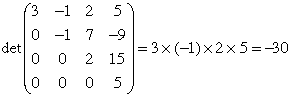
If A is a diagonal matrix, an upper triangular, or a lower
triangular matrix, then det(A) = a1,1a2,2
...an,n. That is, det(A) is the product of the diagonal
elements of A. This is particularly easy to see in the diagonal
case, where only the entries aj,j are not 0. Except for the
term corresponding to the identity permutation in which pk
= k, all of the other terms contain an entry aj,k with j
≠ k. Since such an entry is 0, any term in the determinant that
contains such an entry is also 0. The only term left is
a1,1a2,2 ...an,n. A similar argument
applies to the upper and lower triangular cases as well. We illustrate
this by finding the determinant of a 4×4 upper triangular
matrix.
Fundamental properties of determinants
The properties below follow immediately from the definition. The first three completely characterize
the the determinant; only det(A) satisfies them. The remaining ones are not quite as fundamental, but are still very important.
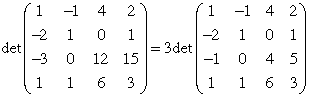
- Homogeneity (Elementary multiplication). A scalar multiplying a single row of a determinant may be factored out. Here is a simple example.
- Elementary modification. A determinant is unchanged if a given row is replaced by the sum of that row and a scalar multiple of another row. In other words, the row operation R = R + cR′ doesn't change a determinant. In the example below, the determinant on the right is obtained from the one on the left by using the row operation R2 = R2 + 2·R1.
- The determinant of the identity matrix is 1. That is, det(I) = 1.
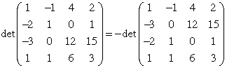
- Row rearrangement (swap). Interchanging two rows changes
the sign of the determinant. In the example below, rows 2 and 3 are
interchanged.
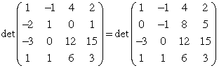
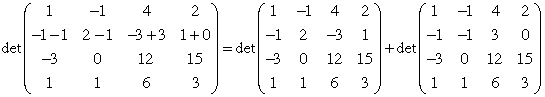
- Additivity. det A is an additive function of a fixed
row. This means that
det([r1; r2;
...; rk + sk;
... rn]) =
det([r1; r2;
...; rk; ... rn]) +
det([r1; r2;
...; sk; ... rn]).
This property is illustrated with the second row in the determinants below.
Useful properties of determinants
There are a number of useful properties one can derive either directly
from the definition or from the list of fundamental properties.
- If a row of A has all 0's, then det(A)=0.
- If two rows of A are equal, then det(A)=0.
- A is invertible if and only if det(A) ≠ 0.
- A is singular if and only if det(A) = 0.
- Product rule
If A and B are n×n matrices, then det(AB)=det(A)det(B).
- det(A-1) = (det(A) )-1
- det(AT) = det(A), so all of the statements above apply
to columns as well as rows.
Cofactor expansions
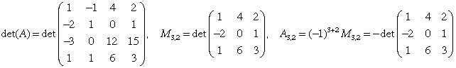
The (i,j) minor Mij for det(A) is the determinant of
the (n-1)×(n-1) matrix formed by removing row i and column j
from A. The (i,j) cofactor Aij for det(A) is defined by Aij = (-1)i+jMij. In the example below, we show the (3,2) minor and cofactor for a 4×4 determinant.
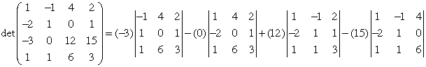
The deteminant of A can be found via expnsion about row i:
det(A) = ΣjaijAij
Similarly, one may use a column expansion:
det(A) = ΣiaijAij
These are nearly identical, except that the summation index is different in the two formulas, the first being over the column index j, and the second over the row index i. The example below is an expansion about row 3. (det(A) = Σja3jA3j.)
Efficient ways of finding determinants
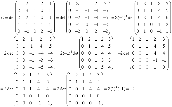
Finding numerical values for determinants of larger matrices is best done using the five properties listed earlier. These properties closely parallel row reduction methods, and can be used in conjunction with them. We will illustrate this by applying it to the determinant of a 5×5 matrix. The idea here is to use row reduction to transform the determinant into upper triangular form, where the answer is then the product of the diagonal entries.
Here is what we did in the steps below. We start with the determinant D. We apply elementary modification to zero out entries below (1,1) in the first column. We then factor three (-1)'s and (-2) out from various rows. The result is the last determinant in the first line. The initial determinant in the second line is obtained by using elementary modification to zero out entries below (2,2). To get the next, we factor out three (-1)'s. the final matrix in the second line is gotten by using elementary modification to zero out the entries below (3,3). We then interchange rows 4 and 5 to arrive at first determinant on the third line. The next determinant, which is upper triangular, is obtained by elementary modification. Since determinants of upper triangular matrices are just products of the diagonal entries, we find D by doing this task.
Cramer's rule
Cramer's rule is a way of writing individual components of the solution to a linear system of equations. This is quite useful in many enginnering applications, where one wants to be able to examine the properties of a the solution when parameters involved are varied. Let A be an n×n matrix, which has the column form A = [a1 ... an]. If A is invertible and Ax = b, then Cramer's rule states that
x1 = det([b a2 ... an])/det(A).
x2 = det([a1 b a3 ... an])/det(A).
...
xn = det([a1 ... an-1 b])/det(A).
Cramer's rule for the inverse of A. Recall that the cofactor Ai,j for the (i,j) entry of A is (-1)i+j Mi,j, where Mi,j is the (i,j) minor that is obtained from A by finding the determinant of the matrix with row i and column j removed. We define the adjugate or classical adjoint of A, which we denote by adj(A), to be the matrix whose (i,j) component is Aj,i. In other words, it is the transpose of the matrix whose entries are the cofactors of A. The formula for the inverse is then
A-1 = adj(A)/det(A).
Updated: 1/30/09 (fjn)