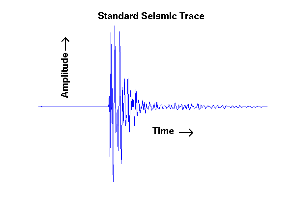
By putting together information from all of the seismic traces, and by using information from holes bored in the ground, they can put together a "picture" of the vertical slice of ground beneath a seismic line. Combining all of these slices then yields a 3D picture of what's below the region's surface.
This process generates enormous amounts of data, and both compressing and analyzing it are very important tasks. The FFT is inadequate here. The reason is that small, high frequency fluctuations are important. Worse, the time when they occur in the the seismic trace is very important, too; it carries information about variations in the rock under ground. Another tool is the short-time Fourier transform. The time interval is broken up into smaller, equal intervals. The FFT is then applied to the data in each interval. This provides some link between time and frequency information, but the equal time intervals cause problems.
In 1983 Grossmann and Morlet, a mathematical physicist and a geophysicist, had the idea of getting around these difficulties with a new transform, one that was better able to analyze and compress seismic traces. They then went on to discover -- actually rediscover, for the mathematician Alberto Calderón had introduced it 1960 in work unrelated to signal analysis -- what is now called the continuous wavelet transform (CWT).
The discrete wavelet transform (DWT) is of more practical interest than the CWT. The first version of it appeared in the early 1900's in work of the Hungarian Alfréd Haar, who was interested in improving on Fourier series by using a different orthogonal set of functions. The basic building blocks were the Haar wavelets. These have many shortcomings, however. It was roughly three quarters of a century later, in the mid-1980's, that discrete wavelets beyond the work of Haar began to be developed. Spurred by the work of Grossmann and Morlet, Meyer, Stromberg, Battle (on our faculty!), Lamarie, Mallat, Daubechies, Chui, and others developed wavelet analysis into a useful tool in applications ranging from image and signal processing to quantum field theory.
The Haar scaling function Discrete wavelet analysis always has two basic functions associated with it. These are the scaling function φ(x) and the wavelet ψ(x).
We will begin with the Haar scaling function, φ(x), which is defined this way: φ(x) = 1 if 0 ≤ x < 1, and φ(x) = 0 otherwise. This is shown in the graph below. By the way, the value of φ at the jump-discontinuities is not important. We picked the ones shown on the graph simply to be definite.

The Haar approximation (scaling) spaces We can approximate a function using a sums of the form ∑kakφ(x-k). The result is roughly the same type of approximation that one uses in connection with Riemann sums. The graph below shows this kind of an approximation for (1+x2)-1 on the interval x = 0 to x = 10.

Of course, we can get a better approximation if we use "thinner" rectangles, just as one would for Riemann sums. For example, if we wanted to use a rectangle having width 1/2 instead of 1, we would start with φ(2x) rather than φ(x). The function φ(2x-1) is φ(2(x-1/2)), or φ(2x) moved to the right 1/2 unit. In fact, φ(2x-k) is φ(2x) moved k/2 units to the right, if k>0, and to the left, if k<0. The approximation that results is shown in the next graph. As you can see, it simply does a better job at approximating the function (1+x2)-2. More graphs are shown in the text in section 4.2.2.

We can adjust the width of rectangles we use use simply by scaling x in φ. The scale factors in discrete wavelet analysis are powers of 2. That is, we can get any width 2-j using φ(2jx). This function is 1 on 0 ≤x < 2-j, and is 0 otherwise. Other "rectangles" are obtained by shifting this basic function. Thus φ(2jx - k) is φ(2jx) shifted to the right 2-jk units if k > 0, and to the left if k < 0.
Approximating with these functions is very important, and so is being able to change the scale 2-j at which we do our approximations. We therefore define the approximation space or scaling space associated with the resolution scale of 2-j to be
Vj = span{...,φ(2jx+2), φ(2jx+1), φ(2jx, φ(2jx-1), φ(2jx -2), ...} = {∑k=-∞∞ akφ(2jx - k)}.
We can also define these spaces directly, without using the scaling function. This is easy to do because of the way the scaling functions φ(2jx - k) themselves are defined, namely 1 on the interval 2-jk ≤ x < 2-j(k+1) and 0 otherwise. If f(x) = ∑k=-∞∞ akφ(2jx - k), then it has to be constant on 2-jk ≤ x < 2-j(k+1), with multiples of 2-j being the only possible discontinuities. In other words, Vj comprises all functions that are piecewise constant, with possible discontinuities occurring at multiples of 2-j.
We close by pointing out two things. The first is that j can be negative. For example, V-1 comprises all functions that are piecewise constant with possible discontinuities occurring only at multiples of 2.
The second thing is that lower resolution approximations also are in the higher resolution spaces. This property is called nesting. In symbols, we write Vj ⊂ Vj+1.To see why, remember that the functions in Vj are constant on intervals 2-jk ≤ x < 2-j(k+1), which include 2-j-1(2k) ≤ x < 2-j-1(2k+1) and 2-j-1(2k+1) ≤ x < 2-j-1(2k+2), so they are in Vj+1. The reader should work this out for the special case in which j = 0, where one wants to show that V0 ⊂ V1.