The bending of polymer bilayers is a mechanism which allows for large deformations via small externally induced lattice mismatches of the underlying materials. This technology recently regained popularity due to new techniques allowing for the fabrication of these materials at the micro scale. Typical applications are thermostats, nanotubes, micro-robots, micro-switches, micro-grippers, micro-scanners, micro-probes, micro-capsules... The proposed reduced model consists of a nonlinear fourth order problem with a pointwise isometry constraint. The bilayer material is modeled as a single plate endowed with an energy proportional to $$ J(y)= \left\lbrace\begin{array}{ll}\frac12 \int_\Omega | II-Z|^2 \ \ \ & \textrm{when } y \textrm{ is an isometry}, \\ +\infty & \textrm{otherwise.} \end{array}\right. $$ Here $II$ denotes the second fundamental form of the plate parametrized by $y:\Omega \rightarrow \mathbb R^3$ and $Z$ is a spontaneous curvature representing the material mismatch.
Equilibrium shapes of bilayer plates for several aspect-ratios $\rho$ (from left to right $\rho=\frac52,\frac32,1,\frac12$) and spontaneous curvatures $Z=-rI_2$ (from top to bottom $r=5,3,1$). Decreasing the aspect ratio restores the ability for the plate to fold into a cylindrical shape for larger spontaneous curvatures. For instance, this is the case for plates with parameters $r=3$ and $\rho=\frac32$ or $r=5$ and $\rho=\frac12$. Notice, however, that small regions around the free corners have not completely relaxed to equilibrium. This effect is due to the violation of the isometry constraint and reduced upon decreasing the discretization parameters as well as the stopping criteria. The numbers below each stationary configuration are the corresponding approximate energies.
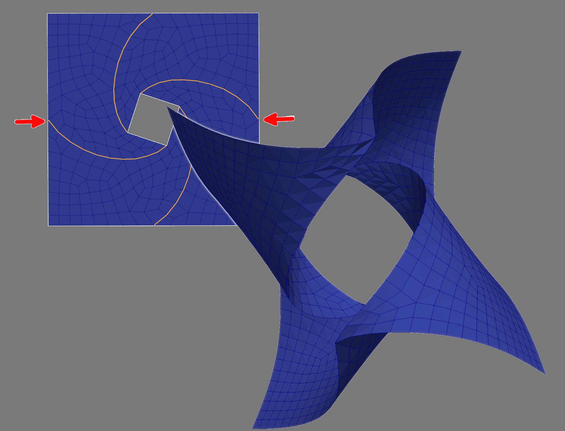
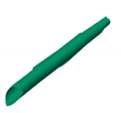
Different snapshots of the deformed corner-clamped plate with spontaneous curvature $Z=-I_2$. The equilibrium shape has energy 11.616 and is not a cylinder. For comparison, the one side fully clamped edge simulation predicts a smaller equilibrium energy (9.81).
Bilayer devices can be used to control the temperature or moisture inside a room. The HygroSkin project by Achim Menges exposed at FRAC Centre Orlean takes advantage of this technology by designing humidity responsive apertures to a pavilion. Heat and moisture are thus dynamically controlled without any high-tech equipment.
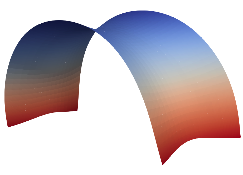
(LEFT) Deformation of a plate with anisotropic curvature given by $$ Z=\begin{pmatrix}1 & 0 \\ 0 & 5 \end{pmatrix}. $$ The spontaneous curvature value is 1 in the clamped direction, its effect being barely noticeable, whereas it is 5 in the orthogonal direction. The equilibrium shape is a cylinder (absolute minimizer) with an energy of 42.09.
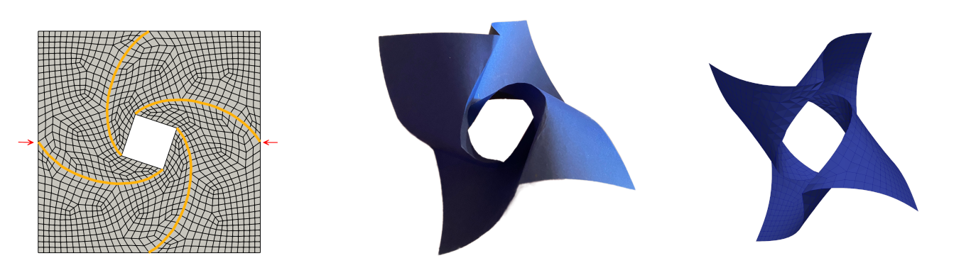
(RIGHT) Deformation of a plate with anisotropic curvature $$ Z=\begin{pmatrix}-3 & 2 \\ 2 & -3 \end{pmatrix}. $$ The principal curvatures are 5 and 1 but the principal directions form an angle $\frac{\pi}4$ with the coordinate axes. The plate adopts a corkscrew shape before self-intersecting.
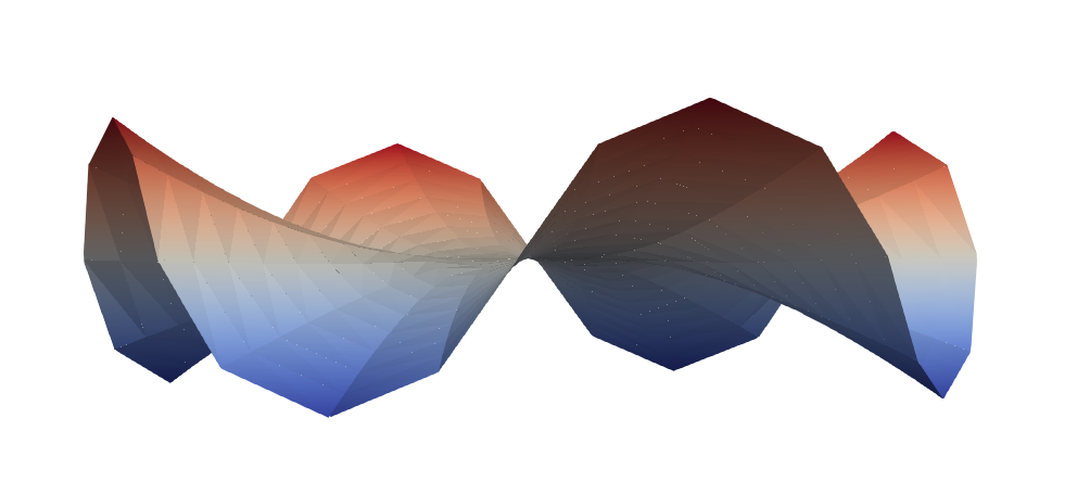
Deformation of a plate with anisotropic curvature given by $$ Z=\begin{pmatrix}5 & 0 \\ 0 & -5 \end{pmatrix}. $$ The spontaneous curvatures are $−5$ in the clamped direction and 5 in the perpendicular direction, which eventually dominates the former and leads to a cylindical shape after three full rotations.
(LEFT) Deformation of a plate with anisotropic curvature given by $$ Z=\begin{pmatrix}1 & 0 \\ 0 & 5 \end{pmatrix}. $$ The spontaneous curvature value is 1 in the clamped direction, its effect being barely noticeable, whereas it is 5 in the orthogonal direction. The equilibrium shape is a cylinder (absolute minimizer) with an energy of 42.09.
(RIGHT) Deformation of a plate with anisotropic curvature $$ Z=\begin{pmatrix}-3 & 2 \\ 2 & -3 \end{pmatrix}. $$ The principal curvatures are 5 and 1 but the principal directions form an angle $\frac{\pi}4$ with the coordinate axes. The plate adopts a corkscrew shape before self-intersecting.
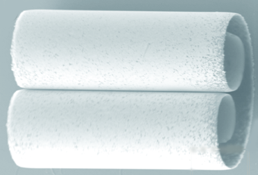

(LEFT) Actual experiment taken from [Alben, Balakrisnan and Smela. Nano letters (2011)] and approximate equilibrium shape with spontaneous curvature $$ Z=\begin{pmatrix}5 & 0 \\ 0 & 0 \end{pmatrix}. $$
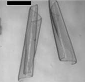
(RIGHT) Actual experiment taken from [Simpson, Nunnery, Tannenbaum, and Kalaitzidou. Journal of Materials Chemistry (2010).] and approximate equilibrium shape with anisotropic curvature $$ Z=\begin{pmatrix}-3 & 2 \\ 2 & -3 \end{pmatrix}. $$
Prestrained thin materials develop internal stresses, deform out of plane, and exhibit nontrivial 3D shapes even without external forces. Chief examples exhibiting such phenomena are nematic glasses, natural growth of soft tissues or manufactured polymer gels. After reduction from 3D to 2D [Battacharya, Lewicka and Shaffner (2016)], denoting by $\Omega\subset\mathbb{R}^2$ the midplane of the plate, the model consists in minimizing the bending energy $$ E(\mathbf{y}) = \frac{\mu}{12}\int_{\Omega}\big|g^{-\frac{1}{2}} \, {\rm II}(\mathbf{y}) \, g^{-\frac{1}{2}}\big|^2+\frac{\lambda}{2\mu+\lambda}{\rm tr}\big(g^{-\frac{1}{2}}\, {\rm II}(\mathbf{y}) \, g^{-\frac{1}{2}} \big)^2 $$ under the constraint that $$\nabla\mathbf{y}^T\nabla\mathbf{y}=g \quad \mbox{a.e. in } \Omega.$$ Here, ${\rm II}(\mathbf{y})$ denote the second fundamental form of the deformed plate $\mathbf{y}(\Omega)$, $\mu$ and $\lambda$ are the Lamé coefficients, and $g$ is the given (symmetric positive definite) target metric. The second fundamental form can actually be replaced by the Hessian of the deformation without affecting the minimizers. In the proposed numerical method, an LDG approach is used for the discretization, where the Hessian is replaced by a so-called discrete Hessian consisting of the broken Hessian and the liftings of jump terms, and an $H^2$ gradient flow is used for the energy minimization.
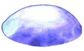
Laboratory manufactured disc gels using an elliptic prestrained metric $g$ (taken from [Sharon and Efrati (2010)]), along with the approximate equilibrium shape.
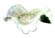
Laboratory manufactured disc gels using a hyperbolic prestrained metric $g$ (taken from [Sharon and Efrati 2010]) along with the approximate equilibrium shape.
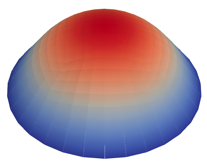
Evolution of the deformation throughout the gradient flow for the unit disc with a positive Gaussian curvature metric.
Evolution of the deformation throughout the gradient flow for the unit disc with a negative Gaussian curvature metric.


Final configurations for the free boundary case with different initial deformations: from left to right, the prestrain defect of the initial deformation is about 2.6, 1.4 and 0.9. The smaller the defect, the closer the final shape is to be a closed catenoid.
Evolution of the deformation throughout the gradient flow. Left: free boundary case; right: view from the side and from the top when boundary conditions for $\nabla\mathbf{y}$ and $\mathbf{y}$ are prescribed on the bottom side of the rectangle.
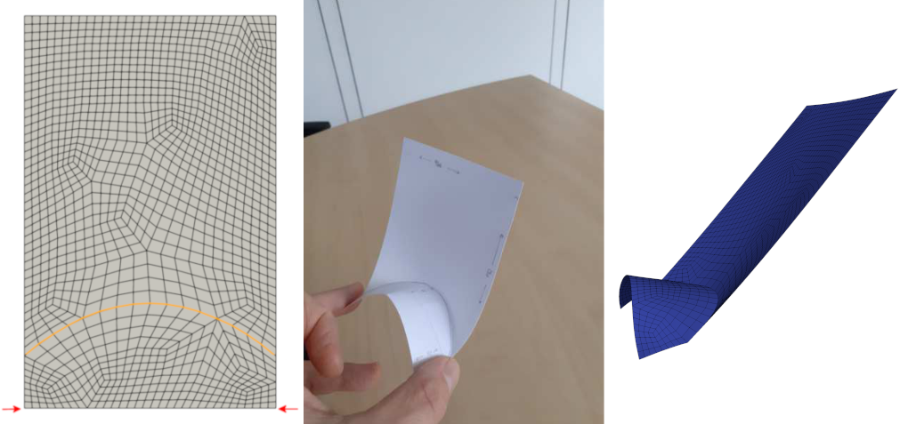
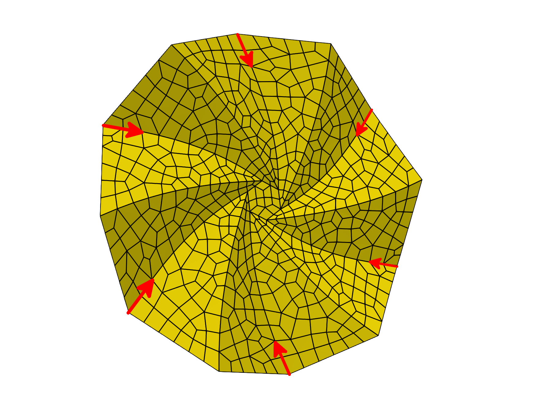
The folding of thin elastic sheets along a prepared curved arc is considered. This naturally leads to bending effects and has recently attracted considerable attention in applied sciences. Particular applications arise in the design of cardboxes and bistable switching devices that make use of corresponding flapping mechanisms. To describe our approach we let $S \subset \mathbb R^2$ be a bounded Lipschitz domain that represents the sheet without thickness and $\Sigma \subset \overline{S}$ be a curve that models the crease, i.e., the arc along which the sheet is folded. The corresponding three-dimensional model involves a thickness parameter $h>0$ and the thin domain $\Omega_h = S \times (-h/2,h/2)$. The material is weakened (or damaged) in a neighbourhood of width $r>0$ around the arc $\Sigma$ and we consider for given functions $W$ and $f_{\epsilon,r}$ the hyperelastic energy functional for a deformation $z:\Omega_h \to \mathbb R^3$ $$ E^h(z) = \int_{\Omega_h} f_{\epsilon,r}(x) |(\nabla z)^T \nabla z - I|^2. $$ Here $f_{\epsilon,r}(x) \in (0,1]$ is small with value $\epsilon>0$ close to the arc $\Sigma$ and approximately $1$ away from the arc. Hence, the factor $f_{\epsilon,r}$ models a reduced elastic response of the material close to $\Sigma$. By appropriately relating the thickness $h$, the intactness fraction $\epsilon$, and width $r$ of the prepared region, we obtain for $(h,\epsilon,r) \to 0$ a meaningful dimensionally reduced model which seeks a minimizing deformation $y:S\to \mathbb R^3$ for the functional $$ E_K(y) = \frac{1}{24} \int_{S \setminus \Sigma} | D^2 y|^2, $$ where $y$ is required to satisfy the pointwise isometry condition \[ (\nabla y)^T (\nabla y) = I. \] Compare with the prestrained or bilayer models described above.
The final configuration of a prestrained plate may depend on the thickness of the plate. The so-called "preasymptotic" model for thin materials accounts for the thickness of the material and allows for the simultaneous bending and stretching of the plate. Denoting the midplane of the plate by $\Omega \subset \mathbb{R}^2$ and the plate thickness by $\theta$, the model consists of minimizing the following bending plus stretching energy: $$ E(\mathbf{y}) = E^S(\mathbf{y})+\theta^2E^B(\mathbf{y}), $$ where the stretching energy $E^S$ is given by $$ E^S(\mathbf{y}) = \frac{1}{8}\int_{\Omega}\left(2\mu\left|g^{-\frac{1}{2}}({\rm I}(\mathbf{y})-g)g^{-\frac{1}{2}}\right|^2+\lambda tr\left(g^{-\frac{1}{2}}({\rm I}(\mathbf{y})-g)g^{-\frac{1}{2}}\right)^2\right) $$ and the bending energy $E^B$ is given by $$ E^B(\mathbf{y}) = \frac{1}{24}\int_{\Omega}\left(2\mu\left|g^{-\frac{1}{2}}{\rm II}(\mathbf{y})g^{-\frac{1}{2}}\right|^2+\frac{2\mu\lambda}{2\mu+\lambda}tr\left(g^{-\frac{1}{2}}{\rm II}(\mathbf{y})g^{-\frac{1}{2}}\right)^2\right). $$ Here, ${\rm II}(\mathbf{y})$ denotes the second fundamental form of the deformed plate $\mathbf{y}(\Omega)$, $\mu$ and $\lambda$ are the Lamé coefficients, and $g$ is the given (symmetric positive definite) target metric. Although not rigorously justified, the second fundamental form can be replaced by the Hessian without significantly affecting the equilibrium deformations. A continuous piecewise polynomial space is used for the the discretization, where the Hessian is replaced by a discrete Hessian consisting of the broken Hessian and the lifting of the jumps of the gradients. An energy-decreasing $H^2$ gradient flow is used for the energy minimization.
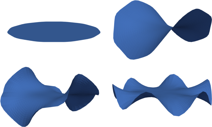
Gel disc experiment with varying thickness. The thickness is given by (left to right and top to bottom) $\theta^2 = 10^{-1}, 10^{-2}, 10^{-3},$ and $0$. More oscillations appear as the thickness decreases, matching experimental results; see Manufactured Gel Disc section.

Evolution of the flapping device as the left end is squeezed. The top row shows the (physically correct) evolution using the preasymptotic model. The bottom row is the evolution using a bending energy with isometry constraint.
When lipid molecules are immersed in aqueous environment they aggregate spontaneously into a bilayers or membrane that forms an encapsulating bag called vesicle. This happens because lipids consist of a hydrophilic head group and a hydrophobic tail, which isolate themselves in the interior of the membrane. This phenomenon is of interest in biophysics because lipid membranes are ubiquitous in biological systems, and an understanding of vesicles provides an important element to understand real cells.
The elastic behavior under large deformations and the dynamics of such deformations are poorly understood. Helfrich in 1973 was one of the first to introduce a model for the equilibrium shape of vesicles where the bending or curvature energy had to be minimized. Jenkins in 1976 arrived to the same model starting from continuum mechanical principles.
The ability to manipulate fluids at the micro-scale is an important tool in the area of bio-medical applications. Micro-fluidic devices often exploit surface tension forces to actuate or control liquids by taking advantage of the large surface-to-volume ratios found at the micro-scale. In particular, some MEMS (micro-electro-mechanical system) devices use electro-wetting which effectively modifies surface tension effects through the use of electric fields, which allows for the manipulation of fluid droplets.
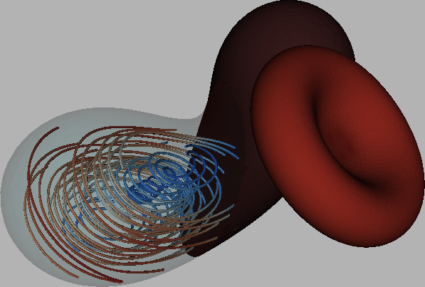
Time evolution of splitting of a droplet. Experiment (blurry line, courtesy Kim's Lab (UCLA)) vs numerical simulation (dashed line).