Theorem. Let V be a vector space with an inner product < u, v >, and let V0 be a subspace of V. A vector v0 in minimizes the distance || v - w || if and only if v0 satisfies the equation,The significance of this theorem is that it provides a way to actually calculate the minimizer. If V0 has an orthonormal basis E = {e1,..., en}, then, since v0 is in V0, we recall that v0 = α1e1 + ... + αnen, where αk = < w0, uk >, k = 1,..., n. By (∗), we have <v - v0, ek > = 0. Thus, <v, uk > = <v0, ek >. From this it follows that αk = <v, uk >, and that the minimizer has the explicit form
(∗) < v - v0, w > = 0,
which holds for all w in V0. In addition, v0 is unique.
v0 = ∑k <v, ek > ek. The important feature of this formula is that we can calculate &appha;k = < v0, ek > without knowing what v0 is. Here are two examples
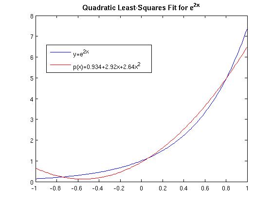
Least squares fitting of a function. We want to find the
quadratic polynomial that gives the best least least squares fit for
the function f(x) = e2x on the interval [-1,1]. In this
case, the inner product and norm are
< f , g > = ∫ −11 f(x)g(x)dx and
||f|| = (∫ −11
f(x)2dx)½.
Since we want to use quadratics, we will take W = P3. The
basis that we will use is E = {p0(x), p1(x),
p3(x)}, where
p0(x) = 2-1/2, p1(x) = (3/2)1/2x, and p2(x)= (5/8)1/2(3x2-1).
These polynomials are called normalized Legendre polynomials and they are orthonormal: <pi, pj> = δij. In this basis, the quadratic polynomial that is the best least squares fit to e2x has the formp(x) = α1p0(x) + α2p(x) + α3p2(x). From our discussion above, we have
α1 = < f, p0> = ∫
−11 e2xp0(x)dx =
8-1/2(e2 - e-2)
&alpha:2 = < f, p1> = ∫
−11 e2xp1(x)dx =
(3/32)1/2(e2 + 3e-2)
α3 = < f, p2> = ∫
−11 e2xp2(x)dx =
(5/128)1/2(e2 - 13e-2)
The quadratic polynomial that is the best least squares fit to
e2x is
p(x) = (1/4)(e2 - e-2) + (3/8)(e2 +
3e-2)x + (5/32)(e2 -
13e-2)(3x2-1).
Both the function and quadratic least squares fit are plotted below.
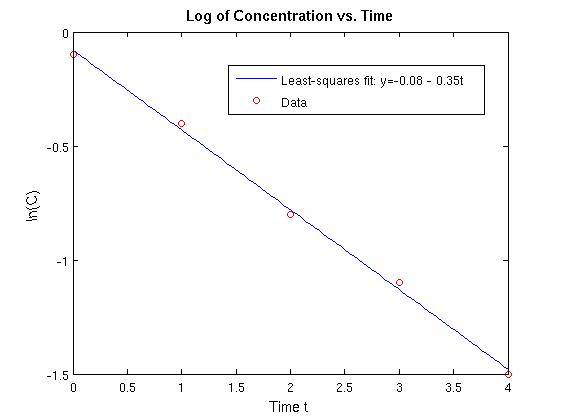
Least-squares data fitting. Problem: The table below contains data obtained by measuring the concentration of a drug in a person's blood. Find and sketch the straight line that best fits the data in the (discrete) least squares sense.
| t | 0 | 1 | 2 | 3 | 4 |
|---|---|---|---|---|---|
| ln(C) | − 0.1 | − 0.4 | − 0.8 | − 1.1 | − 1.5 |
Solution. We want to find coefficients a1 and
a2 such that y = a1 + a2t is the best
least-squares straight-line fit to the data. This means that we choose
the two constants a1 and a2 so that we minimize
the sum S = (y0 − a1 +
a2·0)2 + (y1 −
a1 + a2·1)2 + ... +
(y4 − a1 +
a2·4)2. If we let
w1 = [1 1 1 1 1]T, w2 = [0 1 2 3
4]T, and yd = [-0.1 -0.4 -0.8 -1.1
-1.5]T,
then we can rewrite the sum above in terms of the inner product and
norm for R5:
S = || yd −
a1w1 -
a2w2 ||2
Next, let V0 = span{w1, w2}. The
minimization problem now can be put in the form discussed earlier:
Find v0 in V0 such that || yd − v0 || = minw ∈ V0 || yd − w ||.It is easy to show that if e1 =(5)−½ [1 1 1 1 1]T and e2 = (10)−½;[-2 -1 0 1 2]T, then E = {e1, e2} is an orthonormal basis for V0. The idea here is to first find v0 in terms of the E basis, and then change basis to F = {w1, w2}. The reason for doing this is that a1 and a2 are the just the coordinates of v0 relative to F. In the E basis, v0 = < yd, e1> e1 + < yd, e2> e2 = −(1.7441 u1 + 1.1068 e2). With a little work, we see that e1 = 5−½w1 and e2 = 10−½(w2 − 2w1). Substituting these in the expression for v0 yields
v0 = −0.0800w1 − 0.35w2. From this, we get a1 = −0.08 and a2 = −0.35. The line we want is y = - 0.08 - 0.35t. The data and the line are plotted below.