Math 601 - Fall 2000

Summary

Dates
AUG 29 31              
SEP 5 7 12 14 19 21 26 28  
OCT 3 5 10 12 17 19 24 26 31
NOV 2 7 9 14 16 21 23 28 30
DEC 5                

29 August

Vector spaces
Definition - Vector space. A vector space is a set V together with two operations, + and × . If u, v are in V, then u + v is in V; if c is a scalar, then c×v is in V. The operations satisfy the following rules.

Addition   Scalar multiplication
u + (v + w) = (u + v) + w   a×(b×u) = (ab)×u
Identitiy: u + 0 = 0 + u = u   (a + b)×u = a× u + b×u
Inverse: u + (-u) = (-u) + u = 0   a×(u + v) = a×u + a×v
u + v = v + u   1×u = u

Subspaces
Definition - Subspace. A subset U of V is a subspace if, under + and × from V, U is a vector space in its own right.
Theorem. U is a subspace of V if and only if these hold:
  1. 0 is in U.
  2. U is closed under + .
  3. U is closed under × .
Example: U={(x1, x2, x3) such that x1 + x2 - x3 = 0} is a subspace of R3. On the other hand, W={(x1, x2, x3) such that x1 + x2 - x3 = 3} is not a subspace of R3, because 0 is not in W.

31 August

Span
Definition - Span. Let S={v1 ... vn} be a subset of a vector space V. The span of S is the set of linear combinations of vectors in S. That is,
U=span(S)={c1v1 + ... + cn vn},
where the c's are arbitrary scalars.

Proposition. The set span(S) is a subspace of V.

Dual space

Definition - Dual Space. The set V* of all linear functions f:V - > R (or C) is called the (algebraic) dual of V. Linear means that
f(c1v1 + c2v2) = c1f(v1) + c2f(v2)

Coordinates and Bases

Coordinates for a vector space. The correspondence
v <-> (c1, c2, ... , cn)
should be 1:1, onto, and preserve vector addition and scalar multiplication. If we let vk <-> ek, then the condition of being ``onto'' holds if and only if
V=span{v1, v2, ... , vn}.
The condition of being ``1:1'' holds if and only if {v1, v2, ... , vn} is linearly independent, which we now define.

Definition - Linear independence and linear dependence. We say that a set of vectors
S = {v1, v2, ... , vn}
is linearly independent if the equation
c1v1 + c2v2 + ... + cnvn = 0
has only c1 = c2 = ... = cn = 0 as a solution. If it has solutions different from this one, then the set S is said to be linearly dependent.

Bases

Definition - basis. A subset B = {v1 ... vn} of V is a basis for v if B spans V and is linearly independent. Equivalently, B is a basis if it is maximally linearly independent; that is, B is not a proper subset of some other linearly independent set. Unless we specifically state otherwise, we will assume that B is ordered.

Theorem. Every basis for V has the same number of vectors as every other basis. This common number is defined to be the dimension of V, dim(V).

Coordinates and bases. The properties defining a basis are exactly the ones needed to define ``good'' coordinates for a vector space. Given an ordered basis B = {v1 ... vn} and a vector v, we can uniquely write the vector as v = x1v1 +...+ xnvn, and thus represent it by the column vector [v]B = [x1, ..., xn]T

5 September

Change-of-bases
Let B = {v1 ... vn} and D = {w1 ... wn} be ordered bases for a vector space V. Suppose that we have these formulas for v's in terms of w's and vice versa:

vj=A1jw1 + A2jw2 + ... + Anjwn
wk=C1kv1 + C2kv2 + ... + Cnkvn
(Note that the sums are over the row index for each matrix A and C.) For any vector v with representations
v = b1v1 +...+ bnvn
v = d1w1 +...+ dnwn
and corresponding coordinate vectors
[v]B = [b1,..., bn]T
[v]D = [d1,..., dn]T
we have the change-of-basis formulas
[v]D = A[v]B and [v]B = C[v]D.
These imply that AC=CA=In×n.

Examples

7 September

Inner product
Definition - Inner product Let V be a vector space. we say that a mapping < , > : V×V --> R is an inner product for V if these hold:
  1. positivity - <v ,v > > 0, with <v ,v > = 0 implying that v=0.
  2. symmetry - <u ,v > = <v ,u >
  3. homogeneity - < cu ,v > = c<u ,v >
  4. additivity - < u+v ,w > = <u ,w > + < v, w >

Schwarz's inequality: |<u ,v >| <= ||u|| ||v||, where ||u|| := (<u ,u >)½ is called the norm or length of a vector u.

Triangle inequality: ||u + v|| <= ||u|| + ||v||

12 September

Function spaces - see Function spaces (PS) (PDF)
  • Reviewed inner products; discussed complex inner products
  • Orthogonal sets and orthonormal sets of vectors
  • Separated variables to solve heat equation
    • Discussed solution in terms of inner products; viewed {ei n theta } as an orthonormal set
    • Discussed Cauchy sequences in terms of convergence.
  • Completeness in inner product spaces; all Cauchy sequences converge
  • Hilbert space - a complete inner product space

14 September

Gram-Schmidt Process

Algorithm Let V be a vector space with an inner product < u, v >, and let {v1 ... vn} be a linearly independent set. We want to find an orthonormal set with the same span.

  1. u1 := v1 (|| v1 ||)-1 equivalently v1 = r11u1, r11 = || v1 ||

  2. u2 := (v2 - < v2, u1 > u1) r22-1 equivalently v2 = r12u1 + r22u1,
    where r12 = < v2, u1 > and r22 = || v2 - < v2, u1 > u1 ||

  3. uk := (vk - < vk, u1 > u1 - ... - < vk, uk-1 > uk-1 ) rkk-1 equivalently vk = r1ku1 + ... + rkkuk,
    where rjk = < vk, uj > and rkk = || vk - < vk, u1 > u1 - ... - < vk, uk-1 > uk-1 ||.

  4. Repeat the step above for k = 3, 4, ... n. The result is an orthonormal (o.n.) basis that replaces the vj's.

QR-Algorithm Write all the vj's. and uj's in terms of a common basis, E = {z1 ... zn}. Define the column vectors:
ak = [vk]E and qk [uk]E
Taking coordinates relative to E in the eqaution vk = r1ku1 + ... + rkkuk gives the equation
ak = r1kq1 + ... + rkkqk .
Letting A = [ a1 .. an ], Q = [ q1 .. qn ], and R =
r11 r12  r13  ... r1n
0   r22  r23  ... r2n
0    0   r33  ... r3n
...
0    0   0   ... rnn
we have A = QR. If the basis E doesn't change the inner product, then the columns of Q are orthonormal. This is the QR factorization. It also works if we start with an arbitrary matrix and apply Gram-Schmidt to the column space, with the inner product < u, v > = vTu.

Least-Squares Problem We have a vector v in an inner product space V, and subspace U of V. The least-squares problem is to find the both the minimum of || v - u ||, where u is any vector in U, as well as the minimizer u*.

19 September

Least Squares

Normal equations Let V be a vector space with an inner product < u, v >, and let U be a finite dimensional subspace of V. The vector u* minimizes the distance || v - u || if and only if u* satisfies the normal equations,
< v-u*, u > = 0,
which hold for all u in U. (We say that v - u* is orthogonal to U.)

The minimizer Let U have a basis {w1, ... , wn}. Let u* = c1w1+ ... + cn wn. The normal equations imply that the coefficients xj satisfy the matrix equation

Ac=d,   where Ajk= < wk, wj >,   dj = < v , wj >.

The matrix A is called the Gram matrix for the basis of w's; it is always invertible. (See problem 1, Assignment 4.)

Orthonormal case If the basis {u1, ... , un} (u's replace w's) is orthonormal, then A = I and x = d; that is, the minimizer has the form
u* = < v , u1 > u1+ ... + < v , un > un

Finite element method We want to illustrate the finite element method with a simple example. Solve the ODE - y'' = f(x), y(0) = y(1) = 0. We take the space V to be all continuous functions g(x) defined on [0,1] having a piecewise continuous derivative g'(x) and satisfying g(0) = g(1) = 0. The inner product for this space is < f , g > = S01 f'(x)g'(x) dx. The subspace U comprises all piecewise linear functions in V, with possible discontinuities in the derivatives at 0, 1/n, 2/n, ... (n-1)/n, 1. These are linear B-splines; the possible discontinuities are called knots. A (non-orthogonal) basis is
wj(x) = B(n x - j), j = 1, ..., n-1,
where B(x) is the piecewise linear function defined this way:

B(x) = 0 if x < -1 or x > 1;
B(x) = 1 + x if -1 <= x < 0;
B(x) = 1 - x if 0 < x <= 1.

We want to minimize || y - u ||. Relative to {w1, ... , wn-1}, the normal equations are Ac = d, where
dj = < y, wj > = S01 f(x) wj(x) dx (integrate by parts)
Ajk = < wk, wj >
From here on, one must compute d, A, and solve Ac = d for c. In this case, one can show that u*(x) is just the the piecewise linear function that is 0 at x=0, and cj at x= j/n, j=1, .. , n-1, and 0 at x = 1. One can thus plot u* by ``connecting the dots.'' A specific example will be included in Assignment 4.

Infinite sets of orthonormal vectors See §4 in my notes on Function spaces (PS) (PDF).


21 September

Norms

Definition A norm on a vector space V is a function || || : V -> [0,infinity) that satisfies these properites:
  1. Positivity: || u || >= 0, and || u || = 0 implies u = 0.
  2. Positive homogeneity: || cu || = |c| || u ||
  3. Triangle inequality: || u + v || <= || u || + || v ||

Norms from an inner product || u || = (< u , u1 >)1/2. A norm comes from an inner product if and only if it satisfies the polarization identity. For real vector spaces, this is
|| u + v ||2 + || u - v ||2 = 2(|| u ||2 + || v ||2)

Examples

  1. V = C[a,b], || f || = maxa <= x <= b |f(x)|

  2. V = Rn, || x ||p = (|x1|p + ... + |xn|p)1/p, 1 <= p

  3. V = Rn, || x ||infinity = maxk = 1 ... n |xk|, p = infinity

Linear transformations

Definition A mapping L:V -> W, where V, W are vector spaces is said to be a linear transformation if it satisfies these properties.
  1. Homogeneity L[cu] = cL[u]
  2. Additivity L[u+v] = L[u] + L[v]

Matrix associated with L If V and W are finite dimensional, and if
B = {v1, ... , vn} and D = {w1, ... , wm}
are bases for V and W, respectively, then the matrix for L is an m×n matrix M with columns
Mk = [ L[vk] ]D.
For example, if L=Rt, which rotates a 2D-vector through an angle t, then, using the basis e1 = i, e2 = j, the columns of Mt are
[ Rt[e1] ] = [ cos(t), sin(t)]T
[ Rt[e2] ] = [ -sin(t), cos(t)]T
the the matrix that represents the rotation is
cos(t)  -sin(t) 

sin(t)   cos(t)

26 September

Properties and combinations of linear transformations

Action on linear combinations
L[ c1v1 + c2v2 + ... + cnvn ] = c1L[v1] + c2L[v2] + ... + cnL[vn]

Derivation of the matrix associated with L
Let v = c1v1 + c2v2 + ... + cnvn, so [v]B = [c1, ... , cn]T. From above, we see that

[ L[v] ]D = c1[ L[v1] ]D + c2[ L[v2] ]D + ... + cn[ L[vn] ]D = ML[v]B
where
ML = [ [ L[v1] ]D, ... , [ L[vn] ]D ]

Sums K+L is defined by (K+L)[v] = K[v] + L[v].

Scalar multiples cL is defined by (cL)[v] = c(L[v]).

Products If K : V -> U and L : U -> W are linear, then we define LK via LK[v] = L[K[v]]. (This is composition of functions). The transformation defined this way, LK, is linear, and maps V -> W. Note: LK is not in general equal to KL.

Inverses Let L : V -> V be linear. As a function, if L is both one-to-one and onto, then it has an inverse K V -> V. One can show that K is linear, and LK = KL = I, the identity transformation. We write K = L-1.

Associated matrices

MK + L = MK + ML

McL = c ML

MLK = ML MK

ML-1 = (ML)-1

Polynomials in L : V -> V We define powers of L in the usual way: L2 = LL, L3 = LLL, and so on. A polynomial in L is then the transformation
p(L) = a0I + a1L + ... + amLm
Later on we will encounter the Cayley-Hamilton theorem, which says that if V has dimension n, then there is a degree n (or less) polynomial p for which p(L) is the 0 transformation.


28 September

Change-of-basis

Change-of-basis and linear transformations Let L : V -> V be linear, and let V have bases
B = {v1, ..., vn} and D = {w1, ..., wn}.
If the matrix of L relative to B is ML, and that relative to D is NL, then
NL = SB -> D ML (SB -> D)-1,
where SB -> D changes B coordinates to D coordinates.

Invariant subspaces

Definition Let L : V -> V be linear, and let U be a subspace of V. We say that U is invariant under L if u being in U implies that L[u] is in U.

Eigenvalue problems We say that a scalar l is an eigenvalue of L : V -> V if there is exists a vector v in V, with v not equal to 0, such that L[v] = l v. We let El be the span of all eigenvectors associated with l, and we call El the eigenspace of l. El is an invariant subspace for L.

Characteristic polynomial Let A be an n× n matrix, and define pA(l) = det(A - l I). pA is a polynomial of degree n. The scalar l is an eigenvalue of A if and only if it is a root of pA. This follows from two obeservations: (1) l is an eigenvalue of a if and only if for some x not equal to 0 Ax = l x; this in turn is equivalent to (A - l I)x = 0, so A - l I is singular. (2) A - l I is singular if and only if det(A - l I) = 0.

  • For A, the problem of finding eigenvalues and eigenvectors decouples. One can first find the roots of pA(l), and then solve a linear system to get the eigenvectors.
  • If the scalars are the complex numbers, then the Fundamental Theorem of Algebra implies that pA has at least one root. Consequently, A has at least one eigenvalue.
  • To find the eigenvalues and eigenvectors of a linear transformation L, choose a basis for V and find the matrix of L relative to this basis, ML. The eigenvalues of L are precisely those of ML; the eigenvectors of L have coordinates corresponding to the eigenvectors of ML.

3 October

Determinants - A Quick Tour

Permutations Permutations of the integers 1 through n are either even or odd. A permutation is even if it can be achieved by an even number of interchanges (transpositions), and odd if it takes an odd number of them. There are n! permutaions. We define the function sgn(p) to be +1 if p is an even permutation, and -1 if p is odd.

Definiton of a determinant If A is an n×n matrix, then we define det(A) via
det(A) = SUMp sgn(p) ai1, 1ai2, 2 ...ain, n ,   p = (i1,i2,...,in)

Basic properties of determinants These properties follow immediately from the definition. On the other hand, they characterize the determinant. Only det(A) satisfies them.

  1. Multilinearity. Let A =[a1,a2,...,an]. Then det([a1,a2,...,an]) is a linear function of column ak, if all other columns are held fixed.
  2. Alternating function. Interchanging two columns changes the sign of the determinant.
  3. det(I) = 1, I = identity matrix.

Determinants and matrices
  1. If two columns of A are equal, then det(A)=0.
  2. If a column of A has all 0's, then det(A)=0.
  3. Product rule
    If A and B are n×n matrices, then det(AB)=det(A)det(B).
  4. A is singular if and only if det(A) = 0.
  5. det(A-1) = (det(A))-1

Cramer's rule If A is invertible, and y = Ax, then
x1 = det([y,a2,...,an])/det(A).
x2 = det([a1,y,a3,..., an])/det(A).

...

xn = det([a1,a2,..., an-1, y])/det(A).

Cramer's rule for the inverse of A The cofactor of the (j,k)-entry in A is
Cj,k = det([a1,..,ak-1,ej, ak+1,...,an]]).
The adjugate or classical adjoint of A is adj(A) = CT, and
A-1 = adj(A)/det(A)

Characteristic polynomial
Structure pA(t) = (-1)n tn + (-1)n-1 tn-1 trace(A) + ... + det(A)
Basis independence If B = S-1AS, then pB(t) = pA(t).
Cayley-Hamilton Theorem pA(A) = 0.

5 October

Diagonalization

Definition A linear transformation L : V -> V, where dim(V) = n, is diagonalizable if there is a basis for V relative to which the matrix for L is diagonal.

Matrix Example   The matrix A =
2 -3 1
1 -2 1
1 -3 2
has eigenvalues 0, 1 (repeated twice), and corresponding eigenvectors
{(1,1,1)T}, and {(-1,0,1)T,(3,1,0)T}.
If we let S be the matrix with these eigenvectors as columns - that is, S =
1 -1  3
1  0  1
1  1  0
then S-1 A S =
0  0  0
0  1  0
0  0  1

Lemma   Let L : V -> V have r distinct eigenvalues, and let v1, v2, ..., vr be eigenvectors corresponding to each of the eigenvalues. Then the set of eigenvectors {v1, v2, ..., vr} is linearly independent.

Theorem   Let V be finite dimensional, with n = dim(V). If L : V -> V has n distinct eigenvalues, then L is diagonalizable.

Transformation Example   Let L : P2 - > P2 be given by L[p] = ((1-x2)p')'. L has eigenvalues 0, -2, and -6. Since these are distinct we know that L is diagonalizable. The eigenvectors for L corresponding to 0, -2, and -6 are 1, x, and 3x2-1. These form a basis D = {1, x, 3x2-1} for P2. The matrix for L relative to this basis is the diagonal matrix ML =
0   0   0
0  -2   0
0   0  -6

Non-diagonalizable transformation   Not all linear transformations are diagonalizable. Consider the shear transformation T : R2 -> R2 defined by
T[x] =x + 2x2e1.
The matrix for T is MT =
1 2
0 1
This is not diagonalizable. We can see this directly simply by noting that it has only 1 as an eigenvalue, and for T to be diagonalizable MT would have to be similar to the identity, I. One can also see this by noting that, up to multiples, the only eigenvector is e1, which doesn't form a basis for R2.

10 October

Triangular forms of matrices

Basic upper triangular form   Every matrix A has a basis relative to which it is upper triangular. See Assignment 6, Problem 3.

Block upper triangular form   Every matrix A has a basis relative to which it is in block triangular form. This means that we can find an invertible matrix S such that S-1AS =
T1,1 0 0 ... 0
0 T2,2 0 ... 0
... ... ... ... ...
0 0 0 ...Tr,r
Each diagonal block Tk,k is upper triangular, with the diagonal entries all being an eigenvalue zk repeated as many times as it is a root of the characteristic polynomial. For example, if z7 is repeated four times, then T7,7 =
z7 * * *
0 z7 * *
0 0 z7 *
0 0 0 z7

Jordan normal form   Every matrix A has a basis relative to which the blocks Tk,k are Jordan blocks, Jm(z). This is an m×m matrix with z's down the diagonal, 1's down the superdiagonal, and 0's elsewhere. For example, if m = 6 and z = 3, then J6(3) =
3 1 0 0 00
0 3 1 0 00
0 0 3 1 00
0 0 0 0 3 1
0 0 0 0 0 3
Two matrices having the same Jordan normal form, apart from ordering of the blocks along the diagonal, are similar. An m×m matrix A is similar to Jm(z) if and only there is a basis {f1, ..., fm} satisfying

Af1 = zf1
Af2 = zf2 + f1
...

Afm = zfm + fm-1

Example   Consider the matrix A =
2  1 -1
0  2  3
0  0  2
We begin with the eigenvector, f1 = (1,0,0)T. Solving (A - 2I)f2 = f1 gives f2 = (0,1,0)T. Finally, solving (A - 2I)f3 = f2 gives f3 = (1/3,1/3,0)T. Thus, S-1AS = J3(2), where S = [f1, f2, f3]

Selfadjoint matrices

Adjoints   The adjoint of a linear transformation L : V -> V, where V is an inner product space, is the unique linear transformation L' that satisfies
< L'[u],v > = < u, L[v] > .
For a real m×n matrix A, the adjoint is the transpose AT. If the matrix is complex, then the adjoint of A is AH, the conjugate transpose. A matrix is selfadjoint or Hermitian if it is equal to its own adjoint. Thus, if A is real, A = AT; i.e., A is symmetric.

Properties of selfadjoint matrices
  1. The eigenvalues of a selfadjoint matrix are real.
  2. Eigenvectors corresponding to distinct eigenvalues are orthogonal.
  3. Every selfadjoint matrix is diagonalizable.
  4. Every selfadjoint matrix has an orthonormal basis relative to which it is diagonal. Equivalently, there is an orthogonal matrix S such that STA S is a diagonal matrix. An n×n matrix S is said to be orthogonal if ST = S-1; this amounts to saying that the columns form an orthonormal basis for Rn.

12 October

Singular value decomposition (SVD)

Theorem   Every (real) m×n matrix A can be written as a product A = USVT. Here, U and V are orthogonal matrices, with U being m×m and V being n×n. S is m×n, and has the form S =
s1 0 0 ... 0 ... 0
0 s2 0 ... 0 ... 0
... ... ... ... ... ... ...
0 0 0 ...sr ... 0
0 0 0 ... 0 ... 0
... ... ... ... ... ... ...
0 0 0 ... 0 ... 0
The diagonal entries are positive, and are ordered from greatest to least; r is the rank of A. The sk's are called the singular values of A.

Applications   Gilbert Strang has called this theorem the "Fundamental Theorem of Linear Algebra." The SVD contains very explicit information concerning everything one would want to know about a matrix.

  • Condition number   The condition number of a square, invertible matrix A is defined by
    cond(A) = s1/sn.
    It measures how many significant digits are preserved when one tries to solve Ax = b. For example, if b is known to 6 digits and cond(A) = 103, then x is known to 6 -3 = 3 digits.

  • Numerical rank   The rank of A is r, the number of (positive) singular values. The numerical rank of A is
    rank(A,t) = # of singular values greater than a tolerance t.
    Again, this is useful in working with problems having finite precision.

  • Least squares   The solution to finding a minimum of || Ax - b || is easily done with the SVD. First we rewrite the problem using the SVD for A.
    || Ax - b || = || USVTx -UUT b ||
    || Sz - c ||,   z = VTx   c = UT b

    Then we note that
    || Sz - c ||2 = SUMk = 1...r (skzk - ck )2 + SUMk = r+1...n ck2.

    Choosing zk = ck/sk for k = 1 ... r and zk = 0 for k = r+1 ... n not only solves the problem, but also gives the solution x = Vz with smallest length || x || = || z ||.

Finding the SVD of a matrix   The matrix S above is just the matrix of A relative to new bases for both the input and output spaces.

  • The input space basis   The matrix ATA is real and symmetric, so there is an orthonormal basis of eigenvectors relative to which it is diagonal. Let the eigenvalues of ATA be z1, ..., zn, and the corresponding basis of eigenvectors be {v1, ..., vn}. The eigenvalues are nonnegative, as this calculation shows:

    ATA vk = zk vk
    vkT AT A vk = zk vkT vk
    || A vk ||2 = zk || vk ||2
    || A vk ||2 = zk   (|| vk || =1 )

    This calculation also shows that a vector v is in the null space of A if and only if it is an eigenvecor corresponding to the eigenvalue 0. If r = rank(A), then "rank + nullity = # of columns" tells us that the the nullity(A) = n - r. This means that there are r eigenvectors for the remaining eigenvalues. List these as z1 >= z2 >= ... >= zr > 0. Our input basis is now chosen as {v1, ..., vr, vr+1, ..., vn }. The numbering is the same as that for the eigenvalues. We now define the matrix V via
    V = [ v1 ... vr vr+1 ... vn ].

  • The output space basis   For k = 1, ..., r, let
    uk = A vk / || A vk ||
    uk = A vk / z11/2
    We can also write this as the following equation:
    A vk = zk1/2 uk .
    The uk's are orthonormal, for k = 1, ..., r. Again, we see this from these equations.
    ujT uk = vjT AT A vk / zj1/2 zk1/2
    ujT uk = zk vjT vk / zj1/2 zk1/2
    The orthonormality of the v's implies that the right side above is 0 unless j = k, in which case it is 1. Thus, the u's are orthonormal. Fill this set out with m - r vectors to form an orthonormal basis for the output space, Rm. This gives us the basis {u1, .., ur, ur+1, .., um}. As before, we define the m×m orthogonal matrix
    U = [u1, .., ur, ur+1, .., um].

  • The matrix of A relative to the new bases   We let S be MA. We compute it via the formula for the matrix of a linear transformation.
    S = [ [Av1]U [Av2]U ... [Avr]U [Avr+1]U ... [Avn]U ]
    The v's with k = r+1,...,n, are all in the null space of A. Thus the last n - r vectors are 0, and so are their corresponding columns relative to the basis of u's. The other vectors we get from the definition of the u's for k = 1, ..., r. The end result is this.

    S = [ [z11/2 u1]U [z21/2 u2]U ... [zk1/2 ur]U [ 0 ]U ... [ 0 ]U ]

    S = [ z11/2 [u1]U ... zr1/2 [ur]U   0 ... 0 ]

    S = [ z11/2 e1 ... zr1/2 er 0 ... 0 ].

    If we let sk = zk1/2 for k = 1, ..., r, we get the same S as the one given in the statement of the theorem. These sk's are the singular values of A. The matrix S is related to A via multiplication by change-of-basis matrices. The matrix U changes from new output to old output bases, and V changes from new input to old input bases. Since VT = V-1, we have that VT changes from old input to new input bases. In the end, this gives us A =USVT

Example Consider the matrix A =
 2  -2
 1   1
-2   2
Here, ATA =
 9  -7
-7   9
The eigenvalues of this matrix are z1 = 16 and z2 = 2. The singular values are s1 = 4 and s2 = 21/2. We can immediately write out what S is. We have S =
 4 0
 0 21/2
 0 0
The eigenvector corresponding to 16 is v1 = 2-1/2(1,-1)T, and the one corresponding to 4 is v2 = 2-1/2(1,1)T. Hence, we see that V =
 2-1/2   2-1/2
-2-1/2   2-1/2
Next, we find the u's.

u1 = A v1 / z11/2
u1 = 2-1/2 (4, 0, -4)T/4
u1 =( 2-1/2 , 0, - 2-1/2 )T.

A simlar calculation gives us
u2 =( 0, 1, 0 )T.

We now have to add to these to a "fill" vector
u3 =( 2-1/2 , 0, 2-1/2 )T
to complete the new output basis. This finally yields U =

 2-1/2 0  2-1/2
 0    1  0
-2-1/2 0  2-1/2

17 October

LU Decomposition

Example Let A be an n×n matrix. We want to decompose A into the product of a lower triangular matrix L, which has ones for diagonal elements, and an upper triangular matrix U. Consider the matrix A =
 2 -1 4
  1  1 1
-1  3 2
The highlighted 2 in the first column is the pivot. We perform two row operations to zero-out the rest of the entries in the first column.
R2 = R2 -(1/2)R1
R3 = R3 -(-1/2)R1
These row operations put the matrix into the form below.
2 -1 4
0 3/2 -1
0 5/2 4
We need one last row operation,
R3 = R3 -(2/3)(5/2)R2
     = R3 -(5/3)R2,
to finish finding the matrix U; carrying it out, we get U =
2 -1 4
0 3/2 -1
0 0 17/3
The matrix L is lower triangular and its diagonal elements are 1's. We only need to know the entries LjkRj, where k> j. These turn out to be coefficients involved in the row operations:
Rk = Rk - LjkRj,   k> j.
For our example, L2,1 1/2; L3,1 = -1/2; and L3,2 = 5/3. Hence, L =
  1  0 0
 1/2  1 0
-1/2 5/3 1
One may verify that A = LU. Note that we can read off the determinant of A. The product rule states that det(A) = det(L)det(U) = (13)× (2)(3/2)(17/3) = 17. In general, the determinant of A = LU is simply the product of the pivots, which are the diagonal entries in U.

Review for the Midterm Exam

General information The exam will have five to seven questions, some with multiple parts. The test covers everything we've discussed, except the LU decomposition. You will be asked to state basic definitons, to do simple derivations or proofs (some choice will be given here), and to do problems similar to ones given for homework.

Subspaces Be able to determine whether or not a nonempty subset of a vector space is a subspace.

Change of basis Be able to find the change-of-basis matrix, and be able to change coordinates in vectors and matrices.

Inner products and norms Be able to show Schwarz's inequality and the triangle inequality. Know the terms below and be able to carry out the procedures listed.
  • Orthogonal and orthonormal sets; orthonomal bases; orthogonal matrices
  • Gram-Schmidt procedure
  • QR factorization of a matrix
  • Least squares. Be able to derive the normal equations. Be able to solve the various LS problems that we've discussed.
  • p-norms

Linear transformations Be able to find the matrix of a linear transformation, and be able to find this matrix relative to different bases.

Eigenvalue problems. Be able to find the eigenvalues and eigenvectors for a matrix (or linear transformation).
  • Characteristic polynomial.
  • Cayley-Hamilton Theorem.
  • Diagonalization. Be able to diagonalize a matrix or to explain why it cannot be done.
  • Adjoint of a linear transformation. Diagonalization of selfadjoint matrices by orthogonal matrices. Be able to show that the eigenvalues of a selfadjoint matrix are real, and that eigenvectors corresponding to distinct eigenvalues are orthogonal.
  • Triangular forms. Upper triangular, block upper triangular, and jordan normal form. Know the algorithm for triangularizing a matrix.

Singular value Decomposition. Know what the SVD is, what singular values are, what information the SVD contains, and be able to find it for a simple example.

19 October

Midterm Test

24 October

Multivariate Calculus

Open sets Our functions will be defined on sets that have this simple property: every point in the set can be placed at the center of an n-dimensional ball that is contained entirely in the set. We need this property to discuss limits, derivatives, etc.

Limits We say that limQ -> P f(Q) = L if for every epsilon > 0 there is a delta > 0 such that
|| f(Q) - L || < epsilon   whenever   0 < || P - Q ||< delta . In class we briefly mentioned the reason for using this definition rather than a ``dynamical'' one involving ``P approaching Q''. See The Historical Development of the Calculus, C. H. Edwards, Jr., Springer-Verlag, New York, 1979.

Continuity A function f is continuous at P if limQ -> P f(Q) exists and equals f(P).

Partial derivatives The partial derivative of f : Rn -> Rm with respect to xk is
Dkf(x) = limh -> 0 ( f(x1,...,xk+h,...,xn) - f(x1,...,xk,...,xn))/h

Jacobian derivative If f : Rn -> Rm, so that f(x) = (f1(x), ... , fm(x) )T, then we define the Jacobian derivative of f to be the matrix f´(x) with entries 
f´(x)j,k := Dkfj(x)

Linear approximation If f : Rn -> Rm, then the the linear approximation to f is given by the first two terms on the right below.  
f(x+h) = f(x) + f´(x)h + ||h||eps(h), where eps(h) -> 0 as ||h|| -> 0

Chain rule If g : Rn -> Rp and f : Rp -> Rm, then we let h(x) = f(g(x)). The chain rule states that 
h´(x) = f´(g(x))g´(x)  
Note that the Jacobian derivatives involved are matrices. Order matters! Do not reverse the order in which they are multiplied.

Inverse function theorem Let g : Rn -> Rn. Thus, g takes n variables to n variables, say u = g(w). When can we solve for w in terms of u? That is, when can we find a function h for which w = h(u)? We have to be careful here. We are only looking for an h that works in an open set about u. With that in mind, plus an additional caveat that we are assuming that the functions involved are continuously differentiable, we have that such an h exists when the Jacobian derivative g´(w) is invertible. Moreover, we can calculate h´. It is just given by this:
h´(u) = g´(w)-1, where u = g(w) and w = h(u).

26 October

Tensors

Invariance Physical laws should be formulated in ways that are independent of any coordinates used; that is, the laws should be stated in such a way that they are invariant under transformation of coordinates. For scalar quantities this has a simple meaning. If we know the temperature on a surface T(P) in u-coordinates, so that T=f(u). Then in another coordinate system, u = g(w), the temperature is given by T=f(g(w)). The law of transformation is simply composition of functions (substitution).

Vectors Here is an example of a vector quantity. Suppose that a surface is specified by giving its position x in R3 in terms of parameters u1 and u2; that is, x = x(u1, u2). If a body travels on a curve passing through x at a time t, the velocity vector is
v = a1 f1 + a2 f 2
where
aj = Dtuj and fj = Dujx = partial of x along uj, j=1,2.
If we now change parametrization from u1 and u2 to w1 and w2, where
u = H(w) and w = K(u)
are the functions relating the two sets of parameters, then we can represent the same vector v as
v = b1 g1 + b2 g 2
where
bj = Dtwj and gj = Dwjx = partial of x along wj, j=1,2.
We want to see how various quantities transform under this transformation. Using the chain rule, one can show that
Dwjx = Du1x Dwju1 + Du2x Dwju2.
Equivalently,
gj = H´1,jf1 + H´2,j f2,
where H´ is the Jacobian matrix of H. Quantites that transform with the same coefficients as the ones above are called covariant. To see how the components change, we first note that we are dealing with a change-of-basis problem. Let
F={f1, f2} and G={g1, g2}.
Then, the two coordinate vectors for v are
[v]F = [a1 a2]T and [v]G = [b1 b2]T,
and they transform as follows:
[v]G = (H´)-1[v]F = K´[v]F.
Quantities with components that transform this way are called contravariant.

Dual spaces Let V be an n-dimenasional, real vector space with basis F = {f1,..., fn}. Recall that the dual space of V is the set of all linear functionals v* : V -> R. Corresponding to the basis F for V, we have a dual basis F* = {f*1, ..., f*n} that is defined by the property f*j[fk] = deltaj,k.

31 October

Tensors (continued)

Transformation laws & index notation Recall that we have two types of transformation laws: covariant and contravariant. Objects that transorm covariantly have subscripts. Basis vectors for V transform covariantly, so they are denoted by subscripts, {f1,..., fn}. Dual basis vectors transform contravariantly. Instead of using {f*1,...,f*n} for the dual basis, we will use superscripts {f1,...,f n}. The components for a vector transform contravariantly; thus we use superscripts when working with them. This means that we write a vector v as
v = a1 f1 +... + an fn.
The components of a dual vector transform covariantly, and so we use subscripts for them.
v* = a1 f1 +... + an f n.
We summarize the transformation laws below.

Space Basis Components
V covariant contravariant
V* contravariant covariant


2 November

Examples of Tensors

Stress tensor  By considering the forces on a small tetrahedron, we showed that fn, the contact force per unit area with normal direction n, was a linear function of the components of n. The linear transformation that takes n to fn can be represented by a matrix t jk relative to any given basis E = {e1, e2, e3} for V. Here, we think of the row index as j and the column index as k. The placement of the indices shows how the matrix transforms under a change of coordinates. The quantity t jk is an order 2 mixed type tensor, the stress tensor.

Strain (deformation) tensor  Suppose that a body is deformed so that a point A with coordinates (x1, x2, x3) is moved to a point A´ with coordinates (y1, y2, y3), where
y1 = x1 + u1(x), y2 = x2 + u2(x), y3 = x3 + u3(x).
Consider a point B near to A and having coordinates (x1+ dx1, x2+dx2, x3+dx3). Under the deformation B is moved to B´, which, to first order, has coordinates (y1+dy1, y2+dy2, y3+dy3), where
dyj = dxj+(Dx1uj)dx1 + (Dx2uj)dx2 + (Dx3uj)dx3
The strain tensor measures the change in the distances from A to A´ and from B to B´. If we are working in cartesian coordinates, then the square of the distance from B to B´ is (dy1)2 + (dy2)2 + (dy3)2, and that from A to A´ is (dx1)2 + (dx2)2 + (dx3)2, and the difference between the two is

(dy1)2 + (dy2)2 + (dy3)2 - (dx1)2 -(dx2)2 - (dx3)2 = SUMj,k 2sj,kdxjdxk

where sj,k = ½(Dxjuk + Dxkuj + SUMi DxjuiDxkui) is the strain tensor. (In the linear theory of elasticity, the products are neglected.) The strain tensor is also second order, but it is purely covariant.

Hooke's law In linear elasticity, stress and strain are related via a version of Hooke's law:
t jk = SUMlm c jk,l,m sl,m.
The tensor c jk,l,m is of mixed type and has order 4.

Metric tensor  We had to use cartesian coordinates to find the strain tensor, because we did not have available the distance, or arclength, between nearby points in general coordinates. If we change from cartesian coordinates x to another set w, then the square of the distance between x and x + dx is (ds)2 = (dx1)2 + (dx2)2 + (dx3)2 in cartesian coordinates. Relative to w it becomes

(ds)2 = SUMj,k gj,k dwjdwk.

The tensor gj,k is called the metric tensor. It is purely covariant, and has order 2.


7 November

Change of variables in multiple integrals

Metric tensors and Jacobian determinants  Suppose that we have written the arclength (ds)2 in u-coordinates, so that

In matrix notation, we can write this as (ds)2 = duTgu du. If we now go from u-coordinates to w-coordinates, du = Jdw, where J = is the Jacobian of the transformation u = u(w). since the arclength is an invariant, we have

(ds)2 = dwTJTgu J dw  =   dwTgw dw.
Consequently, we have that gw = JTgu J. This also can be derived via the covariance of the metric tensor. The matrices involved are all square and n×n. Taking the determinants for both sides, and then taking square roots yields

det(gw)1/2 = |det(J)| det(gu )1/2,   J = (w)

The quantity det(J) is called the Jacobian determinant, and is often writtem as

.

Jacobi's Theorem   Consider a change of coordinates x = x(u), where Rx and Ru correspond to each other under it. Then,

Invariant volume   We want to look at the volume element det(gu )1/2du1...dun when we make the change of coordinates u = u(w). First, we have

det(gu )1/2 du1...dun = det(gu )1/2 |det((w))| dw1...dwn.

Recall that we also have det(gw)1/2 = |det(J)| det(gu )1/2,   J = (w). Substituting this into the last equation then gives us

det(gu )1/2 du1...dun = det(gw )1/2 dw1...dwn,

which shows that the combination det(gu )1/2 du1...dun is invariant under coordinate transformations. This is often called the invariant volume element.


9 November

Surface integrals

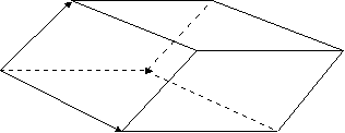
Flux integrals  Consider the steady state velocity field V(x) of a fluid. We want to calculate the amount of fluid crossing a surface parametrized by x = x(u1, u2). Let f1 and f2 be partials of x with respect to the parameters u1and u2. We consider an element of surface area, shown below as the base of the parallelepiped. Our first step is to calculate the fluid crossing this surface element. In time t to t+dt, the volume of fluid crossing the base of the parallelepiped equals its volume, (Vdt)·f1×f2 du1du2.

    Vdt
        f1du1                         f2du2

The mass of the fluid crossing the base in time t to dt is then density×volume, or
Vdt)·f1×f2 du1du2
Thus the mass per unit time crossing the base is F·N du1du2, where F = µV, and N = f1×f2 is the standard normal. Recall that the area of the surface element is dS = |N|du1du2. Consequently the mass per unit time crossing the base is F·n dS, where n is the unit normal. Integrating over the whole surface then yields

This surface integral is called the the flux of the vector field F.


14 November

Three Theorems from Vector Analysis

Curves and Green's Theorem  To state Green's theorem, we need to discuss simple, closed curves. These are closed curves, like circles, but the do not intersect themselves. Rectangles, triangles, circles, and ellipses are simple closed curves; figure eights are not. Simple closed curves divide the plane into two nonoverlapping regions, one interior and the other exterior. It forms the boundary of both regions. We will consider simple closed curves that are piecewise smooth, which just means that we are allowing a finite number of corners. We also say that a simple closed curve is positively oriented if it is travered in the counterclockwise direction. Here is the statement of Green's Theorem:
Green's Theorem Let C be a piecewise smooth simple closed curve that is the boundary of its interior region R. If F(x,y) = A(x,y)i + B(x,y)j is a vector-valued function that is continuously differentiable on and in C, then

The curl and Stokes' Theorem  Let S be a surface in 3D bounded by a simple closed curve C. We will not be absolutely precise here. One should think of S as a butterfly net, with C as its rim. Such a surface is orientable, and we alsways have a consistent piecewise continuous unit normal n defined on S. We say that C is positively oriented if in traversing C with the surface on our left, we are standing in the direction of n.

To state this theorem, we also need to define the curl of a vector field
F(x)=A(x,y,z)i + B(x,y,z)j +C(x,y,z)k.
We will assume that F has continuous partial derivatives. The curl is then defined by


There is an important connection between the Jacobian derivative of a vector field and the curl of that vector field. Namely, the antisymmetric part of the Jacobian derivative has components of the curl for entries.

This is important because it gives us the following formula. For any two vectors b and c in R3,
c T(F-(F')T)b = curl F · b × c .
This is useful in proving Stokes' theorem, which we now state.

Stokes' Theorem  Let S be an orientable surface bounded by a simple closed positively oriented curve C. If F is a continuously differentiable vector-valued function defined in a region containing S, then

The divergence of a vector field and the Divergence Theorem  The divergence of a vector field F(x)=A(x,y,z)i + B(x,y,z)j +C(x,y,z)k is defined by

Like the curl, the divergence of F is connected to the Jacobian derivative F´. Namely, div F = trace(F´), which is the sum of the diagonal entires in F´. We can now state the divergence theorem.

Divergence Theorem  Let V be region in 3D bounded by a closed, piecewise smooth, orientable surface S; let the outward-drawn normal be n. Then,


16 November

Three Theorems from Vector Analysis (cont.)

Verifications  We went over several examples verifying the Diveregnce Theorem and Stokes' Theorem.

Equation of continuity   Let S be a closed surface containing a fluid having velocity v(x,t) and density µ.Assume there are no sources or sinks in S. Let F = µv. The total amount of mass crossing S in the direction of the outward normal is just the flux:

Using the Divergence Theorem, we can write this in terms of a volume integral.

Since there are no sources or sinks in S, any mass entering or leaving the volume enclosed by S must pass through S. Thus, the rate at which mass of fluid inside of S changes in time is the negative of the flux.

Interchanging the time derivative and the triple integral and bringing everything under the same integral, we have that

This equation holds for all regions in which the fluid is source free. It follows that the integrand must be 0, otherwise we could pick a small cube restricted to a region in which it was positive (or negative). The whole integral would then be positive (or negative). Hence, we arrive at the following equation, known as the equation of continuity:


21 November

PDEs of mathematical physics

Derivation of the Heat Equation  See § VI.2 in Zachmanoglou and Thoe (Z/T). The steady state version of this equation is Laplace's equation.

Separation of variables

Dirichlet problem for Laplace's equation in the disk  See § VII.2, VII.7 in Z/T.

28 November

Fourier series

Expansions in Fourier series  See § VII.8 in Z/T.
Solution to Dirichlet problem  See § VII.7 and VII.8 in Z/T.

Vibrating string with ends clamped

Solution via separation of variables See § VIII.8 in Z/T.
Sine series See § VII.8 and § VIII.8 in Z/T.

30 November

Vibrations in Finite Regions

Separation of variables See VIII.10 in Z/T.
Eigenfunction expansions See VIII.10, Theorem 10.1.
Vibrations in a circular membrane See VIII.10, Example 10.3.

5 December

D'Alembert's Solution to the Wave Equation

One dimensional case  Change variables in uxx- utt=0 from x and t to p=x+t and q=x-t. The result is upq=0. Integrating, we have u=F(p)+G(q), or u(x,t)=F(x+t)+G(x-t). See § VIII.2 for the rest of the solution.

Three dimensional radial case  See §VIII.1.

Divergence, Laplacian, and Curl in General Coordinates and Spherical Coordinates

Divergence

Laplacian

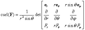
Curl

Review for the Final Exam

General information The exam will have six to eight questions, some with multiple parts. The test will cover the material discussed after the midterm exam; there will be no direct questions on material prior to the midterm. You will be asked to state basic definitons and theorems, to do simple derivations or verifications, and to do problems similar to ones given for homework. The specific topics covered are as follows:

Multivariate Calculus
  • Jacobian derivative
  • Chain rule
  • Inverse function theorem

Tensors

Change of variables in multiple integrals
  • Jacobi's Theorem.

Surface integrals  See my notes on surfaces.
  • Area element
  • Normals - unit and standard
  • Flux and density integrals
  • Parametrizations of simple surfaces

Green's Theorem, Divergence Theorem, Stokes' Theorem

Partial differential equations.
  • Initial value and boundary value problems. See Z/T VI.2.
  • Separation of variables.
    • Laplace's equation in the disk. See § VII.2, § VII.7.
    • Fourier series. See § VII.8.
    • Vibrating string. See § VIII.8.
    • Vibrating drumhead. See § VIII.10.
    • Eigenvalue problems and eigenfunction expansions. See § VIII.10
  • D'Almebert's solution to the one-dimensional wave equation.