|
|
Easiest (and smallest)
|
| |
This first model was designed by
D. Henderson in conjunction with
Cabinet Magazine.
Here are some on-line
instructions.
For this, you may want to print out one
instruction sheet,
and you will need three
templates.
This is the first model in our gallery.
Taping the unprinted side
gives a neater model and facilitates the mathematics activity below.
Using tape (such as Scotch tape) that can be written on is a good idea.
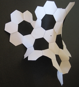
I suggest one improvement to this model.
The irregular-shaped pieces each include one distinguished hexagon with a black dot in its
center, and the instructions ask you to attach three together on top of each other, forming
the center of your model.
I recommend cutting this hexagon off two of the three templates and taping the remaining
part of the templates to the remaining central hexagon.
| |
|
|
|
Another Model, used in Sottile's activities
|
| |
This has fairly big (3 cm on a side) polygons and can be used to make a
fairly big model.
It is important to use high-quality paper and be very
careful with the taping, for the inherent stresses in a big model can tear the paper.
Print out what you need on white paper.
I prefer extremely bright and thick paper.
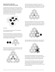
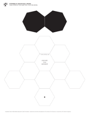
You need one copy of the center (HF_Center.pdf) and one or two copies of the side
(HF_Side.pdf).
Cut only on the dotted lines, and cut out the heptagons.
Tape a heptagon in the central hole of the center (HF_Center.pdf); in doing this the
hexagonal ring will open up,
and there is room for an additional hexagon. Use the one you cut from the hole.
The hexagons will form a ring around the heptagon, and on the outside of this ring are
several indentations formed by three hexagons.
Tape in two heptagons in two of these that are side-by-side.
Then the strip of seven hexagons in the side (HF_Side.pdf) may be attached onto them.
Your model will be almost symmetrical with three heptagons surrounding a central
hexagon and surrounded by a ring of 15 hexagons, with one additional hexagon breaking
the symmetry.
If you wish, you can tape in the five remaining heptagons on the periphery of this
model for a complete and slightly asymmetrical piece of hyperbolic paper.
The third sheet contains three patterns of four hexagons each for attaching to these
new heptagons, allowing a larger model.
| |
|
|
|
Biggest and most extensible
|
| |
This has the biggest polygons, and can be used to make a
fairly big model.
To make a big model, it is important to use high-quality paper and be very
careful with the taping, for the inherent stresses in a big model can tear the paper.
Print out what you need on white paper.
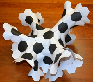
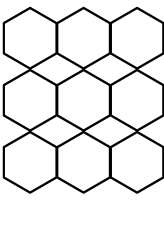
Three copies of Template A (Hyperbolic_Football_A.pdf) mak an interesting
model that is identical to Henderson's model.
You must cut on the dotted lines, and the central hexagon should be removed whole (there is
a cut to it), as one will be needed at the centre of this model.
To add more to your model, print out as many of whichever of the templates as you need.
Note that Template C has two extra hexagons that you will want to cut out and use in your
model.
| |
|
|
|
Most cutting
(but with color)
|
| |
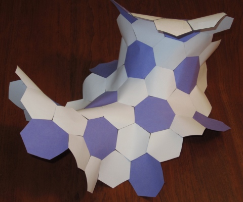
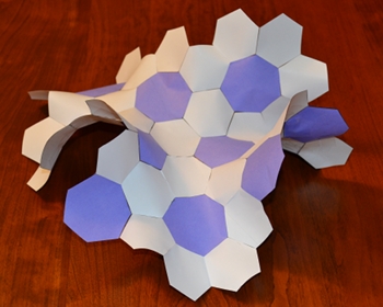
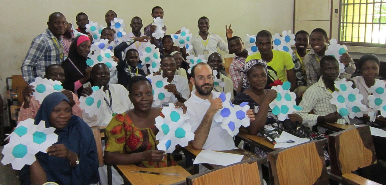
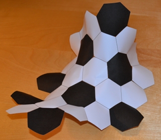
This model is depicted above with the purple heptagons.
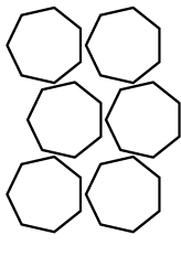
Print the heptagons (7-sided figures) on coloured paper, and hexagons on white paper.
Use the same printer, and try to have the ratio heptagons:hexagons close to 3:7.
Carefully cut out the figures, and tape them together (put tape on the printed side of the
paper to get a neater model).
Each heptagon is taped to seven hexagons, and each hexagon to three heptagons and three
hexagons, alternating.
(See the pictures above.)
| |
|
|
Mathematical activities with your model
|
Drawing a line
Begin with any of the above models, although using a big one is
extremely cumbersome.
At right is the last model above, from the 2013 Joint Mathematics Meetings.
Turn it over and write on the back (the unprinted side).
While this model is curved, each polygon is flat (it was cut from a
single piece of paper).
Also, any two adjacent polygons can be laid flat.
To draw a line on the model, flatten part of the model to start the line, and use a
short (< 15 cm) straightedge to continue the line across the model, flattening
pairs of polygons as needed.
Try to avoid running the line through a vertex.
After drawing your line completely across the model, you can pick it up,
straighten it along the line, and sight down the line to see that it is straight.
Viewing it from above, it appears to curve, but that is an illusion as it is drawn on
a curved surface.
|
|
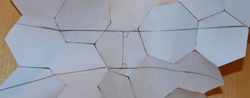
Diverging Parallels
After drawing a first line, pick a point on it and draw a short line
segment m perpendicular to it.
Then start a new line perpendicular to m and extend this third line across the
model.
The first and third lines, as they share a common perpendicular m, are
parallel.
If m is long enough, say nearly the height of a hexagon as at right, then you
should be able to notice the interesting feature that the two lines appear to `curve'
apart.
They do not curve, but the distance between them increases the further they get from
the common perpendicular m, which is their only common perpendicular.
This divergence is more pronounced for a longer common perpendicular m.
|
|
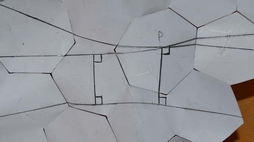
The Parallel Postulate and a Lambert Quadrilateral
Euclid's parallel postulate,
(or rather its equivalent Playfair's axiom), states that:
At most one line can be drawn through any point not on a given line parallel to the
given line in a plane.
This is easily seen to not hold on the hyperbolic plane.
Indeed, on one of the parallel lines from the previous step, choose a point P
not lying on the common perpendicular m.
Dropping a perpendicular from P to the other line, and then taking a
perpendicular to that through P gives a second line through P that is
parallel to the original line.
The two original parallels and two perpendiculars together form a
Lambert Quadrilateral
which has three right angles and one acute angle (at P).
|
|
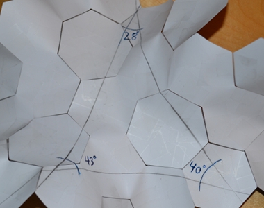
Triangles
Now, try to draw a triangle.
For this it is best to try to make a big triangle.
Once you are done, measure its angles.
This is easier said than done, as you cannot fit a protractor on the hyperbolic paper.
I prefer to mark off an arc on a small sector of a circle (cut out of a scrap of paper),
lay the semicircle on a flat surface, and then use my protractor.
However you do it, you should find that the angles have a sum that is
less than 180°.
For example, in the triangle at right, that the sum is less than 180° is visually
immediate.
In fact, the angles were measured to be 43°, 40°, and 28°,
for an angle sum of 111°, plus-or-minus some measurement error.
It is possible to use an analog measurement of the sum.
Simply mark off three consecutive arcs along a small sector of a circle, then the sum
should be apparently less than 180°.
This is nice to do in a group, for different participants will make different
triangles, and you can discuss the different angle sums that they get.
|
|
Curvature
We explain what is the meaning of the angle sum (and also what
is the acute angle in our Lambert quadrilateral above).
If you have really careful participants, this can be a
fascinating discovery activity.
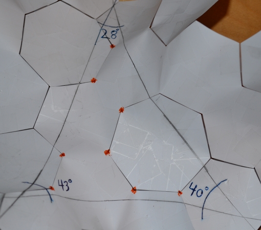
We remarked that the model is mostly flat.
In fact, its curvature is concentrated at the vertices, where two hexagons and one
heptagon meet.
The sum of the angles at that vertex is
vertex ∠ hexagon + vertex ∠ hexagon + vertex ∠ heptagon
= 120° + 120° + (180°-360/7°)
= 360° + 60/7°.
Thus there is an excess of 60/7°, which is about 8.6°.
By convention, we say that the curvature at each vertex is -8.6°, which we
consider to be a δ function, as the curvature everywhere else is zero.
Thus the integral of the curvature over a region is -8.6N°,
where N is the number of vertices in that region.
There are 8 vertices in our triangle, so the integral of the curvature
over the triangle is 8 times -8.6°, which is about -68.6°, and is almost
exactly the deviation of our angle sum (111°) from the Euclidean triangle angle
sum of 180°.
This is of course not a coincidence, but an example of the general
theorem.
This has several consequences.
First, our Lambert quadrilateral has acute angle (90-60/7)°, which is about
81.4°.
Far more fascinating, which you can see on a large model, is that a triangle cannot contain
21 or more vertices (3 heptagons).
I have collected data on this from several classes of students.
These are displayed and described on the page Triangles in hyperbolic space
|
|