Proposed VIGRE Seminar Spring 2001
Asymptotic and Numerical Approaches
to Spectral and PDE Problems
(This was not adopted as a VIGRE course, but a modified version
will run as independent study (Math. 485/685).)
Professors Stephen Fulling, Jianxin Zhou, Alexei
Poltoratski
This seminar will be concerned with the behavior of basic
solutions (Green functions) of partial differential equations
in certain limits.
The central themes will be:
- solve PDEs by eigenfunction expansions;
- try to learn something interesting about the solutions.
There are implications in physics:
- heat conduction, diffusion
- geometrical optics
- classical limit of quantum mechanics
- vacuum energy (Casimir effect)
- effects of chaos
Concrete, explicit examples
are valuable in
improving understanding of the
implications of the general theory.
Asymptotic methods and numerical
methods need to be employed together.
This is an area where students can make meaningful contributions
before mastering the upper levels of abstract theory.
In more mathematical terms, we are dealing with a field variously known
as "spectral asymptotics", "spectral geometry", or "semiclassical
approximation". It is the study of relationships between the "geometry"
of a differential operator, such as
L = -(1/2)Laplacian + V(x)
-- for example, the region of space where L acts, the boundary
conditions, and the lengths of the closed orbits of the corresponding ODE
system,
d2x/dt2 = - grad V(x)
-- and the "spectral apparatus" of L (eigenvalues,
eigenfunctions, etc.). Usually these connections are discovered by
investigating a third class of objects, the integral kernels (Green
functions) that solve various PDEs associated with L.
Here is a sampling of questions related to this seminar,
ranging from easy and solved problems to hard problems that
will probably be unsolved when we end.
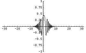
- Oscillatory integrals. Suppose that you need to
evaluate numerically an integral of the form
(in Maple lingo)
Int( cos((x-y)2) g(y) , -infinity .. infinity)
and plot it as a function of x.
If g(y) = exp(-16*(y-0.5)2), we know that the right answer
should look like this:
 But a numerical integration gave this:
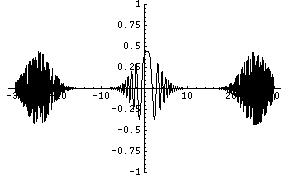 What is causing the junk on the sides? How might you get rid of it?
Here is a document showing Mathematica code and further commentary
for this problem:
(DVI version ._.
PostScript version ._.
PDF version)
(This problem is about 3/4 solved.)
What is causing the junk on the sides? How might you get rid of it?
Here is a document showing Mathematica code and further commentary
for this problem:
(DVI version ._.
PostScript version ._.
PDF version)
(This problem is about 3/4 solved.)
- Global effects of boundary conditions.
- How could you tell whether our world has a mirror at one end
(a surface where u(t,0)=0)?
Would you rather solve
- the heat equation, du/dt = d2u/dx2, or
- Laplace's equation,
d2u/dt2 + d2u/dx2 = 0 ?
[Hint]
- Suppose that our world is a circle and the the quantity u(t,x)
"lives on a Moebius strip",
so that u(t,2*pi) = - u(t,0).
Could we detect this from solutions of the heat equation or Laplace's
equation?
(This problem has been solved, with
undergraduate student assistance.
(PDF version)
Here is more information
on this question.
Green function for the Schrodinger equation on a circle.
Does the sum
Sum( cos(t*k2), k= -infinity, infinity) /(2*pi)
converge? Let's study the convergent sum
Sum( exp(-p*k2)*cos(t*k2), k= -infinity, infinity) /(2*pi)
where p is a very small positive number (called the "cutoff").
(Here is a
more detailed explanation of these computations:
DVI version ._.
PostScript version ._.
PDF version.)
Here is the result with p = 0.1:
Now let's take p closer to zero (0.01):
Hmm, the graph just seems to be getting more complicated.
Let's take a close-up:
And now try a smaller value of p (0.001):
Notice the change in vertical scale!
Is this function going to approach a limit as p goes
to zero? Let's look even closer up:
And take p still smaller (0.0001):
Notice the spike suspiciously close to t = pi/2. Looking back at the
earlier graphs, do you see something special happening at other
multiples of pi by simple rational numbers?
Here is a complete Maple session
devoted to this problem; the examples above are taken from the
second half of it.
(These phenomena have been understood by number theorists for generations,
but most physicists have never heard of them, even though the function
describes the simplest quantum system, a particle in a one-dimensional
periodic box.)
Extracting asymptotics from a numerical solution.
Consider the PDE d2u/dt2 +
d2u/dx2 - x2u = 0 on a rectangle
with the values of u(t,x) prescribed on the four boundaries.
In particular, u(0,x) = 0.
- Can we solve this problem numerically?
(Yes, this can be done by standard techniques.)
- From the numerical solution, can we reliably extract
the values of du(0,x)/dt ?
(This question has not yet been seriously addressed.
It is one of the things we need to investigate.)
WKB-type solutions.
Can we find approximate paper-and-pencil (not numerical) solutions
to equations like the one above,
d2u/dt2 + d2u/dx2
- x2u = 0 ?
What if the - x2 is replaced by 1/cosh2(x) ?
(This problem is solved in principle, but some work is needed to apply
the solution in our context.)
Resonances in a constant electric field.
This is another undergraduate student project that became a published
paper.
See C. E. Dean and S. A. Fulling, "Continuum eigenfunction expansions
and resonances: A simple model", American Journal of Physics
50, 540-544 (1982) (unfortunately, before the Web).
Traces of classical chaos in the Casimir effect.
Quantum theory predicts the existence of "vacuum energy"
inside a perfectly reflecting cavity.
If the cavity is very symmetrical (like a sphere),
the classical rays trace out very regular patterns.
If the cavity is very bumpy, the rays wander around the
cavity in a chaotic fashion.
Is there a qualitative difference in the vacuum energy,
depending on whether the rays are regular or chaotic?
Some general arguments suggest that the effect should be
smaller in the chaotic case;
but some experiments suggest the exact opposite.
(This is a hard problem. We will barely scratch the surface
of it in this seminar.)
You need not think that these questions are easy --
just that they are interesting!
Prerequisites:
- Ordinary differential equations (Math. 308 or 451)
- Linear algebra (Math. 311 or 423)
-
Previous exposure to partial differential equations and eigenfunction
expansions (such as Fourier series) (Math. 312 or similar)
will be very helpful but not required.
Much of the first two weeks of the course will be devoted to providing this
background material.